Plotting

gplot draws a network as a layered, top-down graph: roots on the first row, every other node one row below its deepest parent, with edges attached to the exact border of each shape. It works on any network — a BayesianNetwork, CredalNetwork, or EnhancedBayesianNetwork — and on a DirectAcyclicGraph, so a structure can be inspected before its parameters are even learned.

W = DiscreteNode(:W)
W[:W => :sunny] = 0.7
W[:W => :rainy] = 0.3
U = ContinuousNode(:U, [:W])
U[:W => :sunny] = Normal()
U[:W => :rainy] = Normal(2, 1)

net = EnhancedBayesianNetwork([W, U])
add_child!(net, W, U)
order!(net)

gplot(net; title = "weather", legend = true, background_color="white")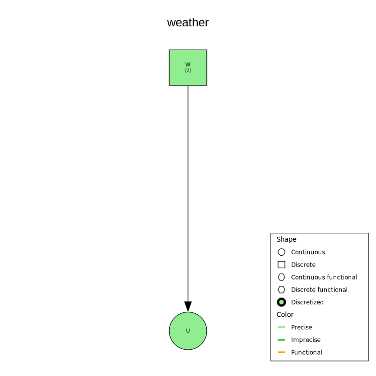

The visual language

The drawing encodes each node's kind, precision, and discretization, so the diagram doubles as a summary of the model:

Encoding	Meaning
Rectangle	discrete node
Circle	continuous node
Pointy hexagon	discrete functional node
Rounded hexagon	continuous functional node
Pale fill	precise node
Bright fill	imprecise node
Orange fill	functional node
Thick border	continuous node carrying a discretization

Discrete nodes also show their number of states below the name. Pass legend = true to draw the shape/colour key on the canvas (positioned by legend_x and legend_y, as fractions of the canvas).

Customizing the drawing

gplot takes keyword arguments to size and annotate the figure:

• title, title_scale — a title above the graph and its font scale.

• node_scale — scale every node shape up or down.

• label_scale — scale the node-label font independently of the shapes.

• figsize — the canvas size, a tuple of Compose measures (e.g. (20cm, 20cm), the default).

• legend, legend_scale, legend_x, legend_y — toggle, scale, and position the legend.

gplot(net; title = "weather", node_scale = 1.2, label_scale = 0.9, figsize = (16cm, 12cm))

Saving to a file

gplot returns a Compose.Context. saveplot writes it to an SVG file:

p = gplot(net; title = "weather", legend = true)
saveplot(p, "weather.svg")