Metamodels

Linear Basis Function Models

Linear basis function models are a simple class of metamodels that express the predicted output as a linear combination of basis functions evaluated for the input variables defined as

$$y(\mathbf{x})=\sum _{i=1}^n{\beta }_i{\phi }_i(\mathbf{x}),$$

where ${\phi }_i(x)$ are nonlinear basis functions that map the input space into an intermediate feature space and $\beta$ represents the adjustable weights. Some commonly used basis functions are introduced next.

Monomial Basis

Monomial basis functions are defined as the powers, or products of powers in the multivariate case, of the input variables with a total degree of less than or equal to $d$. For example, the monomial basis in two variables of degree $d=3$ in graded reverse lexicographic order is given by

$$\phi (x)=[1,x_2,x_1,x_2^2,x_1{x}_2,x_1^2,x_2^3,x_1{x}_2^2,x_1^2{x}_2,x_1^3]$$

The construction of this MonomialBasis is presented next.

φ = MonomialBasis(2, 3)

MonomialBasis(2, 3, Monomials.Monomial[1, x2, x1, x2², x1x2, x1², x2³, x1x2², x1²x2, x1³])

By default the MonomialBasis includes the constant (zero degree) term. This behaviour can be changed by passing the include_zero=false keyword.

Radial Basis

A radial basis function (RBF) is a real-valued function $\phi (||\mathbf{x}-\mathbf{c}||)$ that depends on the distance between the input $\mathbf{x}$ and a fixed point $\mathbf{c}$, called a center. These functions are multivariate but reduce to scalar functions of the radius $r=||\mathbf{x}-\mathbf{c}||$, hence the name radial basis function. The distance used is most commonly the euclidian norm. UncertaintyQuantification provides two types of RBFs.

Gaussian

$$\phi (r)=\exp (-ϵr)$$

here, $ϵ$ is a shape parameter. Gaussian radial basis functions are exposed through the GaussianRadialBasis struct.

Polyharmonic

$$\phi (r)=\{\begin{array}{lll}{r}^k& \text{with}& k=1,3,5,\dots ,\\ r^k\ln (r)& \text{with}& k=2,4,6,\dots \end{array}$$

Note, that polyharmonic radial basis functions do not require a shape parameter. These RBs can be constructed using the PolyharmonicRadialBasis type.

Least Squares

Despite the nonlinearity of the basis functions, the model remains linear in its parameters, which allows efficient estimation of the weights using ordinary least squares. Given $m$ observations $({\mathbf{x}}_i,y_i)$, for $i=1,\dots ,m$ we construct the design matrix $\mathrm{\Phi }$ where each row contains the evaluated basis functions for one input:

$${\mathrm{\Phi }}_{ij}={\phi }_j({\mathbf{x}}_i),\text{ for }i=1,\dots ,n\text{ and }j=1,\dots ,m$$

The optimal weight vector is found by minimizing the sum-of-squares error

$$E(\beta )=\sum _{i=1}^m(y({\mathbf{x}}_i,\beta )-y_i{)}^2$$

yielding the closed-form solution via

$$\beta =({\mathrm{\Phi }}^{\mathrm{\top }}\mathrm{\Phi }{)}^{-1}{\mathrm{\Phi }}^{\mathrm{\top }}\mathbf{y},$$

where $\mathbf{y}$ is the output vector.

Example

Consider the function

$$y(x)=x\cos (x),$$

where $x\sim U(-5,5)$

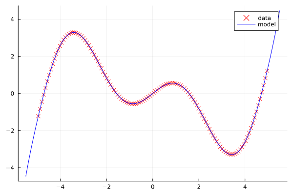
We use HaltonSampling to sample 150 data points from the input variable, evaluate the model, and fit a LinearBasisFunctionModel using a MonomialBasis of degree $d=9$.

x = RandomVariable(Uniform(-5, 5), :x)
y = Model(
        df -> df.x .* cos.(df.x),
        :y,
    )
data = sample(x, HaltonSampling(150))
evaluate!(y, data)
lbfm = LinearBasisFunctionModel(data, :y, MonomialBasis(1, 9))

ResponseSurface(MonomialBasis(1, 9, Monomials.Monomial[1, x1, x1², x1³, x1⁴, x1⁵, x1⁶, x1⁷, x1⁸, x1⁹]), [0.00018241593646902075, 0.9878644609495059, -0.00018150970456987044, -0.48925985169682223, 4.747249404303626e-5, 0.038987490233917725, -3.913393749589379e-6, -0.0011115728398402001, 9.668870671278248e-8, 1.1603496934147144e-5], [:x], :y)

A plot comparing the resulting model to the data points is presented next.

Response Surface

A linear basis function model constructed from a MonomialBasis is also known as a polynomial Response Surface [31]. For this reason we provide a convenient alias ResponseSurface. Using this alias the previous example can be adapted as follows.

rs = ResponseSurface(data, :y, 9)

ResponseSurface(MonomialBasis(1, 9, Monomials.Monomial[1, x1, x1², x1³, x1⁴, x1⁵, x1⁶, x1⁷, x1⁸, x1⁹]), [0.00018241593646902075, 0.9878644609495059, -0.00018150970456987044, -0.48925985169682223, 4.747249404303626e-5, 0.038987490233917725, -3.913393749589379e-6, -0.0011115728398402001, 9.668870671278248e-8, 1.1603496934147144e-5], [:x], :y)

Design Of Experiments

Several experimental designs have been developed to efficiently estimate ResponseSurface models [31]. Although designed for response surface methodology these designs can be used to fit any metamodel. However, for more complex models we suggest using Quasi Monte Carlo sampling schemes instead.

The designs implemented in UncertaintyQuantification are TwoLevelFactorial, FullFactorial, FractionalFactorial, CentralComposite, BoxBehnken, and PlackettBurman.

Interval Predictor Model

An interval predictor model (IPM)[32] is a function that returns an interval instead of a precise value for the dependent variable given as

$$I_y(x,P)=\{y=p^T\phi (x),p\in P\},$$

where $\phi (x)$ is an arbitrary basis and the uncertainty set $P$ is defined as

$$P=\{p:\underset{―}{p}\le p\le \bar{p}\}.$$

Using the defining vertices of P $\underset{―}{p}$ and $\bar{p}$ the IPM results as

$$I_y(x,P)=[\underset{―}{y}(x,\bar{p},\underset{―}{p}),\bar{y}(x,\bar{p},\underset{―}{p})],$$

with

$$\underset{―}{y}(x,\bar{p},\underset{―}{p})={\bar{p}}^T\left(\frac{\phi (x)-|\phi (x)|}{2}\right)+{\underset{―}{p}}^T\left(\frac{\phi (x)+|\phi (x)|}{2}\right)$$

and

$$\bar{y}(x,\bar{p},\underset{―}{p})={\bar{p}}^T\left(\frac{\phi (x)+|\phi (x)|}{2}\right)+{\underset{―}{p}}^T\left(\frac{\phi (x)-|\phi (x)|}{2}\right).$$

Here, $\underset{―}{y}$ and $\bar{y}$ are the lower and upper bounds of the IPM.

The distance between the lower and upper bound given by

$${\delta }_y(x,\bar{p},\underset{―}{p})=(\bar{p}-\underset{―}{p}{)}^T|\phi (x)|$$

is known as the spread of the IPM. The optimal defining vertices for a given data set are found by minimizing the average spread such that all data points fall into the IPM by solving the following convex constrained optimization problem.

$$\{\underset{―}{p},\bar{p}\}=\underset{u,v}{\mathrm{argmax}}\{{\mathbb{E}}_x[{\delta }_y(x,u,v]:\underset{―}{y}(x_i,v,u)\le y_i\le \bar{y}(x_i,v,u),u\le v\}$$

Example

Consider the function

$$y(x)=x^2\cos (x)-\sin (3x)\exp (-x^2)-x-\cos (x^2)+xg,$$

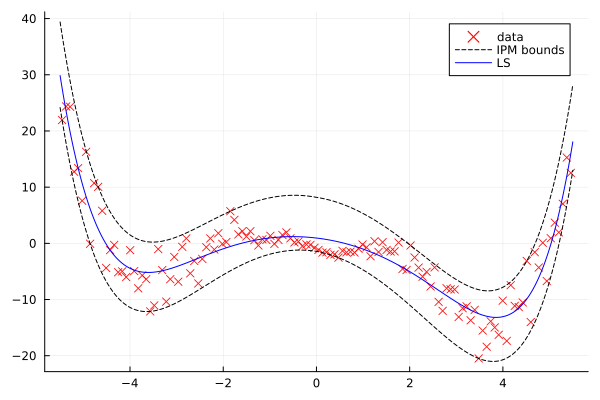
where $x\sim U(-5.5,5.5$ and $g\sim N(0,1)$. We generate a data sequence of $N=150$ points and fit an IntervalPredictorModel using a MonomialBasis of sixth degree.

x = RandomVariable(Uniform(-5.5, 5.5), :x)
data = sample(x, HaltonSampling(150))

m = Model(
        df ->
            df.x .^ 2 .* cos.(df.x) .- sin.(3 * df.x) .* exp.(-df.x .^ 2) .- df.x .-
            cos.(df.x .^ 2) .+ df.x .* randn(size(df, 1)),
        :y,
    )

evaluate!(m, data)

b = MonomialBasis(1,6)
ipm = IntervalPredictorModel(data, :y, b)

IntervalPredictorModel{MonomialBasis}(MonomialBasis(1, 6, Monomials.Monomial[1, x1, x1², x1³, x1⁴, x1⁵, x1⁶]), [-1.917225644166731, -1.7765048387513835, -0.9899778933490903, 0.05447606704122796, -0.04630799524392712, -0.001956415232260404, 0.003457335796681521], [6.970384634890219, -0.8018186415622978, -0.9899778933489536, 0.05447606704123612, -0.04630799524392633, -0.001956415232260114, 0.0037807639963089814], [:x], :y, 150)

The following figure presents the bounds of the resulting IPM and the corresponding least squares solution. Note, that the least squares solution is not guaranteed to be between the bounds of the IPM.

IPM reliability

The reliability of the IPM, that is the probability that and unobserved data point $(x,y)$ will fall in the interval $I_y(x,P)$ can be assessed using the reliability function. The function reliability(ipm, ϵ) returns the confidence parameter $\beta$. Then, the reliability of the IPM is no less than $1-ϵ$ with confidence $1-\beta$.

1 - reliability(ipm, 0.1548)

0.9898502075787752

Reliability analysis

As the IPM is an imprecise model, it can only be applied in a reliability analysis using the DoubleLoop or RandomSlicing. For more information, see Imprecise Reliability Analysis.