Simulations

Monte Carlo

The Monte-Carlo (MC) method is a method of sampling random numbers that dates back to 1777. The name was suggested by Nick Metropolis when MC was used while working on the Manhattan Project. It is used in Random Number Generators which generally produce pseudo random numbers. Extensive information on the Monte-Carlo method can be found in [33].

Quasi Monte Carlo

For a comprehensive introduction to Quasi Monte Carlo, view [34]. The following provides an essential overview.

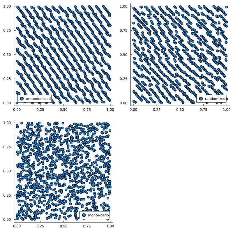
Quasi Monte Carlo (QMC), is a method of producing samples similar to those generated via Monte Carlo (MC). The difference being that QMC samples are generated deterministically in a way to ensure they are evenly distributed across the sampling space, not forming clutters or voids as MC samples might. This makes QMC more efficient than MC for lots of applications, since fewer samples are needed in order to produce a sufficient density of samples throughout. There are multiple ways of QMC sampling methods which can be classified as either digital nets/sequences or lattices [35]. Since the samples are not random, they are not suitable for many tasks. However, it is possible to randomize QMC samples by randomly shifting or scrambling each sample.

While the disjunction of a deterministic sampling and a randomization method that can be applied to the samples later is most common for QMC, there are also some sampling methods that directly produce quasi random samples.

Dependency QuasiMonteCarlo.jl

This package relies on QuasiMonteCarlo.jl which offers various QMC sampling methods as well as corresponding randomization methods. An example on how to use them is shown below.

The package provides the following deterministic sampling algorithms:

• Lattices:

  • GridSample

  • LatticeRuleSample

  • GoldenSample

  • KroneckerSample

• Digital nets:

  • SobolSample

  • FaureSample

  • HaltonSample

Note

KroneckerSample should not be used with bases > 3. GoldenSample is a special version of a KroneckerSample and should be used with base 1 only. Otherwise, LatticeRuleSample is the preferred method. For more information on this and on the implementation of the other sampling algorithms, please consult the corresponding documentation of QuasiMonteCarlo.jl.

Note

The number of samples for digital nets should always be a power of the base, while lattices work best with large prime numbers as sample-sizes. Straying from these rules may worsen results significantly, since the samples will be imbalanced [36].

The samples can be randomized by shifting using these methods:

• Shift (Cranley-Patterson rotation [37])

• Scrambles:

  • MatousekScramble[38]

  • OwenScramble[39] or

  • DigitalShift(functions similarly to Shift, but takes the base that was used during sampling into account)

Note

For randomizing lattice-samples, Shift is recommended. The mentioned scrambling methods work well with samples from digital nets.

Further, these are the available randomized sampling algorithms: * LatinHypercubeSample[40] * RandomizedHaltonSample[41]

Example

To facilitate QMC-sampling in UncertaintyQuantification.jl one needs to first create one or more random variables to sample from as well as an instance of QuasiMonteCarloSampling, which takes the number of samples and the desired sampling algorithm from QuasiMonteCarlo.jl. Using the sample-function, the defined number of samples is created from the given variable(s).

    using QuasiMonteCarlo
    x = RandomVariable(Uniform(), :x)
    qmc = QuasiMonteCarloSampling(128, LatinHypercubeSample())
    samples = UncertaintyQuantification.sample(x, qmc)

It is of course possible to directly create the QuasiMonteCarloSampling-instance inside the sample-call, enabling a more efficient version of the example above which looks like this:

    x = RandomVariable(Uniform(), :x)
    samples = UncertaintyQuantification.sample(x, QuasiMonteCarloSampling(128, LatinHypercubeSample()))

Note

When chosing n, be reminded that, for digital nets, n must be a power of the base that is used for creating the respective sequence. For SobolSample the base is always equal to 2 while for FaureSample, it depends on the number of input-variables, being the smallest prime number that is greater or equal to the number of variables.

    x = RandomVariable(Uniform(), :x)
    samples = UncertaintyQuantification.sample(x, QuasiMonteCarloSampling(128, QuasiMonteCarlo.SobolSample()))

128×1 DataFrame

Row	x
	Float64
1	0.0117187
2	0.511719
3	0.761719
4	0.261719
5	0.386719
6	0.886719
7	0.636719
8	0.136719
9	0.199219
10	0.699219
11	0.949219
12	0.449219
13	0.324219
14	0.824219
15	0.574219
16	0.0742188
17	0.105469
18	0.605469
19	0.855469
20	0.355469
21	0.480469
22	0.980469
23	0.730469
24	0.230469
25	0.167969
26	0.667969
27	0.917969
28	0.417969
29	0.292969
30	0.792969
31	0.542969
32	0.0429687
33	0.0585938
34	0.558594
35	0.808594
36	0.308594
37	0.433594
38	0.933594
39	0.683594
40	0.183594
41	0.246094
42	0.746094
43	0.996094
44	0.496094
45	0.371094
46	0.871094
47	0.621094
48	0.121094
49	0.0898437
50	0.589844
51	0.839844
52	0.339844
53	0.464844
54	0.964844
55	0.714844
56	0.214844
57	0.152344
58	0.652344
59	0.902344
60	0.402344
61	0.277344
62	0.777344
63	0.527344
64	0.0273437
65	0.0195312
66	0.519531
67	0.769531
68	0.269531
69	0.394531
70	0.894531
71	0.644531
72	0.144531
73	0.207031
74	0.707031
75	0.957031
76	0.457031
77	0.332031
78	0.832031
79	0.582031
80	0.0820313
81	0.113281
82	0.613281
83	0.863281
84	0.363281
85	0.488281
86	0.988281
87	0.738281
88	0.238281
89	0.175781
90	0.675781
91	0.925781
92	0.425781
93	0.300781
94	0.800781
95	0.550781
96	0.0507812
97	0.0351562
98	0.535156
99	0.785156
100	0.285156
101	0.410156
102	0.910156
103	0.660156
104	0.160156
105	0.222656
106	0.722656
107	0.972656
108	0.472656
109	0.347656
110	0.847656
111	0.597656
112	0.0976562
113	0.0664063
114	0.566406
115	0.816406
116	0.316406
117	0.441406
118	0.941406
119	0.691406
120	0.191406
121	0.128906
122	0.628906
123	0.878906
124	0.378906
125	0.253906
126	0.753906
127	0.503906
128	0.00390625

To emphasize the importance of randomization, consider the correlations that might occur using unrandomized QMC and how they are fixed by randomizing. For instance, this is the 7th dimension plotted against the 8th in Faure Sampling, unrandomized vs. randomized via Owen Scramble: