Gaussian Process Regression
Himmelblau's Function
In this example, we will model the following test function (known as Himmelblau's function) in the range
It is defined as:
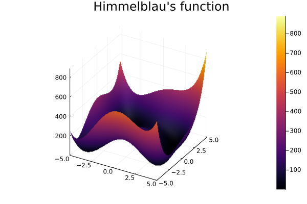 Analogue to the response surface example, we create an array of random variables, that will be used when evaluating the points that our experimental design produces.
using UncertaintyQuantification

x = RandomVariable.(Uniform(-5, 5), [:x1, :x2])

himmelblau = Model(
    df -> (df.x1 .^ 2 .+ df.x2 .- 11) .^ 2 .+ (df.x1 .+ df.x2 .^ 2 .- 7) .^ 2, :y
)
Next, we chose a experimental design. In this example, we are using a LatinHyperCube design from which we draw 80 samples to train our model:
design = LatinHypercubeSampling(80)LatinHypercubeSampling(80)After that, we construct a prior GP model. Here we assume a constant mean of 0.0 and a squared exponential kernel with automatic relevance determination (ARD). We also assume a small Gaussian noise term in the observations for numerical stability:
mean_f = ConstMean(0.0)
kernel = SqExponentialKernel()

gp_prior = GP(mean_f, kernel)
GP{ConstMean{Float64}, SqExponentialKernel{Distances.Euclidean}}(ConstMean{Float64}(0.0), Squared Exponential Kernel (metric = Distances.Euclidean(0.0)))Next, we set up an optimizer used in the log marginal likelihood maximization to find the optimal hyperparameters of our GP model. Here we use the Adam optimizer from the Optim.jl package with a learning rate of 0.005 and run it for 10 iterations.:
using Optim

optimizer = MaximumLikelihoodEstimation(Optim.Adam(alpha = 0.005), Optim.Options(; iterations = 10, show_trace = false))
Finally, we define an input standardization (here a z-score transform). While not strictly necessary for this example, standardization can help finding good hyperparameters. Note that we can also define an output transform to scale the output for training the GP. When evaluating the GP model, the input will be automatically transformed with the fitted standardization. The output will be transformed back to the original scale automatically as well.
input_transform = ZScoreTransformChoice()The GP regression model is now constructed by calling the GaussianProcess constructor with the prior GP, the input random variables, the model, the output symbol, the experimental design, and the optional input and output transform choices. The construction then samples the experimental design, evaluates the model at the sampled points, standardizes the input and output data, and constructs the posterior GP.
gp_model = GaussianProcess(
    gp_prior,
    x,
    himmelblau,
    :y;
    experimental_design = design,
    input_transform = input_transform,
    optimizer = optimizer
)
The GP regression model uses finite projections of the fitted posterior GP to make predictions. As of now, the hyperparameters of the GP might not be optimal. We can find optimal hyperparameters through maximizing the log marginal likelihood of observing the training data under the posterior GP.
To evaluate the GaussianProcess, use evaluate!(gp::GaussianProcess, data::DataFrame) with the DataFrame containing the points you want to evaluate. The evaluation of a GP is not unique, and we can choose to evaluate the mean prediction, the prediction variance, a combination of both, or draw samples from the posterior distribution. The default is to evaluate the mean prediction. We can specify the evaluation mode via the mode keyword argument. Supported options are:
:mean- predictive mean (default):var- predictive variance:mean_and_var- both mean and variance:sample- random samples from the predictive distribution
test_data = sample(x, 1000)
evaluate!(gp_model, test_data; mode = :mean_and_var)
The mean prediction of our model in this case has an mse of about 65 and looks like this in comparison to the original:
s1 = surface(a, b, himmelblau_values; plot_title="Himmelblau's function")
s2 = surface(a, b, gp_mean; plot_title="GP posterior mean")
plot(s1, s2, layout = (1, 2), legend = false)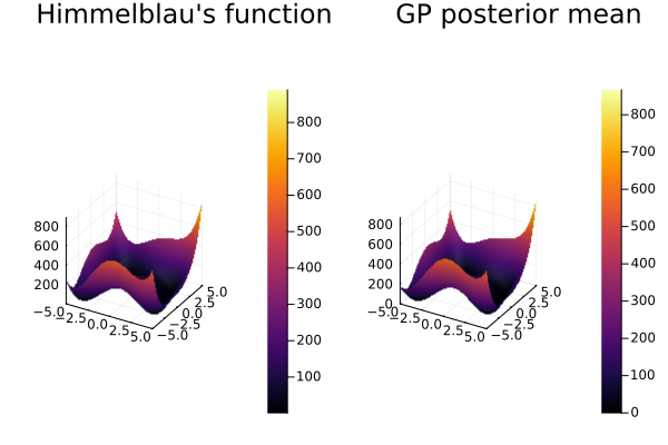
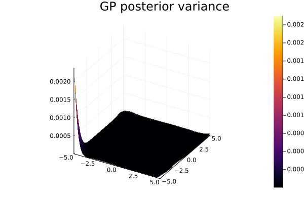
Note that the mse in comparison to the response surface model (with an mse of about 1e-26) is significantly higher. However, the GP model also provides a measure of uncertainty in its predictions via the predictive variance.
Adaptive Gaussian Process Regression
Adaptive Gaussian process regression enriches an initial surrogate model with new evaluations selected by a learning function. At every iteration, the algorithm samples candidate points, selects the most informative one according to the learning function, evaluates the expensive model there, and refits the Gaussian process.
Himmelblau's Function
As in the (non-adaptive) GP example, we consider the Himmelblau function in
First, define the probabilistic input and the expensive model to approximate.
x = RandomVariable.(Uniform(-5, 5), [:x1, :x2])
himmelblau = Model(
    df -> (df.x1 .^ 2 .+ df.x2 .- 11) .^ 2 .+ (df.x1 .+ df.x2 .^ 2 .- 7) .^ 2, :y
)
We start with the same initial Gaussian process surrogate as in the regular GP regression example. Hence, we use the same initial design and same optimizer.
design = LatinHypercubeSampling(80)
mean_f = ConstMean(0.0)
kernel = SqExponentialKernel()

gp_prior = GP(mean_f, kernel)
input_transform = ZScoreTransformChoice()
optimizer = MaximumLikelihoodEstimation(Optim.Adam(alpha = 0.005), Optim.Options(; iterations = 10, show_trace = false))

initial_gp = GaussianProcess(
    gp_prior,
    x,
    himmelblau,
    :y;
    experimental_design = design,
    input_transform = input_transform,
    optimizer = optimizer
)
Next, we update the initial GP using a selected learning function and a set number of additional points used to refine the initial GP. We use the MaximinDistance acquisition function and select 20 additional points.
learning_function = MaximinDistance()
n_added_points = 20
We refine the GP using AdaptiveGaussianProcess which we pass our initial GP, the learning_function and n_added_points.
adaptive_gp = AdaptiveGaussianProcess(
    deepcopy(initial_gp),
    x,
    himmelblau,
    learning_function,
    n_added_points;
    optimizer = optimizer
)
To assess the fitted surrogate, we compute the MSE between GP mean and the reference model. We compare the MSE of the initial GP and the refined GP.
We start with the initial GP:
test_data = sample(x, LatinHypercubeSampling(1000))
test_data_adaptive = deepcopy(test_data)
evaluate!(initial_gp, test_data; mode = :mean)
evaluate!(himmelblau, test_data)

mse = mean((test_data.y .- test_data.y_mean) .^ 2)
println("MSE (initial GP):  $mse")
MSE (initial GP): 9.532185802172158Then, we also evaluate the adaptively refined GP at the same test set:
evaluate!(adaptive_gp, test_data_adaptive; mode = :mean)
evaluate!(himmelblau, test_data_adaptive)

mse_adap = mean((test_data_adaptive.y .- test_data_adaptive.y_mean) .^ 2)
println("MSE (adaptive GP):  $mse_adap")
MSE (adaptive GP): 0.7549453669845093Metamodels
Design Of Experiments
Design Of Experiments (DOE) offers various designs that can be used for creating a model of a given system. The core idea is to evaluate significant points of the system in order to obtain a sufficient model while keeping the effort to achieve this relatively low. Depending on the parameters, their individual importance and interconnections, different designs may be adequate.
The ones implemented here are TwoLevelFactorial, FullFactorial, FractionalFactorial, CentralComposite and BoxBehnken.
Response Surface
A Response Surface is a structure used for modeling. It can be trained by providing it with evaluated points of a function. It will then, using polynomial regression, compute a model of that function.
Example
In this example, we will model the following test function (known as Himmelblau's function)
in the range
At first we need to create an array of random variables, that will be used when evaluating the points that our design produces. It will also define the range of the function we want the design to fit. This is also a good time to declare the function that we are working with.
using UncertaintyQuantification

x = RandomVariable.(Uniform(-5, 5), [:x1, :x2])

himmelblau = Model(
    df -> (df.x1 .^ 2 .+ df.x2 .- 11) .^ 2 .+ (df.x1 .+ df.x2 .^ 2 .- 7) .^ 2, :y
)
Model(Main.var"#8#9"(), :y)Our next step is to chose the design we want to use and if required, set the parameters to the values we need or want. In this example, we are using a FullFactorial design:
design = FullFactorial([5, 5])FullFactorial([5, 5], 0.99)After that, we call the sample function with our design. This produces a matrix containing the points of our design fitted to the range defined via the RandomVariables. Wer then evaluate the function we want to model in these points and use the resulting data to train a ResponseSurface. The ResponseSurface uses regression to fit a polynomial function to the given datapoints. That functions degree is set as an Integer in the constructor.
Note
The choice of the degree and the design and its parameters may be crucial to obtaining a sufficient model.
training_data = sample(x, design)
evaluate!(himmelblau, training_data)
rs = ResponseSurface(training_data, :y, 4)

test_data = sample(x, 1000)
evaluate!(rs, test_data)
To evaluate the ResponseSurfaceuse evaluate!(rs::ResponseSurface, data::DataFrame) with the DataFrame containing the points you want to evaluate.
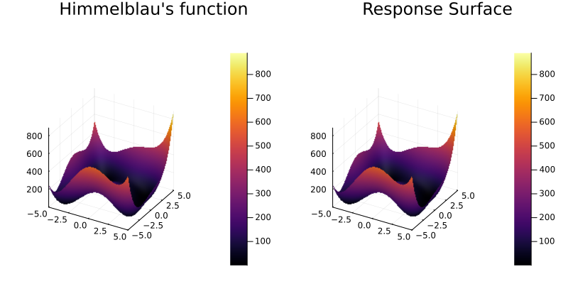
The model in this case has an mse of about 1e-26 and looks like this in comparison to the original:
This page was generated using Literate.jl.