Metamodels

Linear Basis Function Models

Linear basis function models are a simple class of metamodels that express the predicted output as a linear combination of basis functions evaluated for the input variables defined as

$$y(\mathbf{x})=\sum _{i=1}^n{\beta }_i{\phi }_i(\mathbf{x}),$$

where ${\phi }_i(x)$ are nonlinear basis functions that map the input space into an intermediate feature space and $\beta$ represents the adjustable weights. Some commonly used basis functions are introduced next.

Monomial Basis

Monomial basis functions are defined as the powers, or products of powers in the multivariate case, of the input variables with a total degree of less than or equal to $d$. For example, the monomial basis in two variables of degree $d=3$ in graded reverse lexicographic order is given by

$$\phi (x)=[1,x_2,x_1,x_2^2,x_1{x}_2,x_1^2,x_2^3,x_1{x}_2^2,x_1^2{x}_2,x_1^3]$$

The construction of this MonomialBasis is presented next.

φ = MonomialBasis(2, 3)

MonomialBasis(2, 3, Monomials.Monomial[1, x2, x1, x2², x1x2, x1², x2³, x1x2², x1²x2, x1³])

By default the MonomialBasis includes the constant (zero degree) term. This behaviour can be changed by passing the include_zero=false keyword.

Radial Basis

A radial basis function (RBF) is a real-valued function $\phi (||\mathbf{x}-\mathbf{c}||)$ that depends on the distance between the input $\mathbf{x}$ and a fixed point $\mathbf{c}$, called a center. These functions are multivariate but reduce to scalar functions of the radius $r=||\mathbf{x}-\mathbf{c}||$, hence the name radial basis function. The distance used is most commonly the euclidian norm. UncertaintyQuantification provides two types of RBFs.

Gaussian

$$\phi (r)=\exp (-ϵr)$$

here, $ϵ$ is a shape parameter. Gaussian radial basis functions are exposed through the GaussianRadialBasis struct.

Polyharmonic

$$\phi (r)=\{\begin{array}{lll}{r}^k& \text{with}& k=1,3,5,\dots ,\\ r^k\ln (r)& \text{with}& k=2,4,6,\dots \end{array}$$

Note, that polyharmonic radial basis functions do not require a shape parameter. These RBs can be constructed using the PolyharmonicRadialBasis type.

Least Squares

Despite the nonlinearity of the basis functions, the model remains linear in its parameters, which allows efficient estimation of the weights using ordinary least squares. Given $m$ observations $({\mathbf{x}}_i,y_i)$, for $i=1,\dots ,m$ we construct the design matrix $\mathrm{\Phi }$ where each row contains the evaluated basis functions for one input:

$${\mathrm{\Phi }}_{ij}={\phi }_j({\mathbf{x}}_i),\text{ for }i=1,\dots ,n\text{ and }j=1,\dots ,m$$

The optimal weight vector is found by minimizing the sum-of-squares error

$$E(\beta )=\sum _{i=1}^m(y({\mathbf{x}}_i,\beta )-y_i{)}^2$$

yielding the closed-form solution via

$$\beta =({\mathrm{\Phi }}^{\mathrm{\top }}\mathrm{\Phi }{)}^{-1}{\mathrm{\Phi }}^{\mathrm{\top }}\mathbf{y},$$

where $\mathbf{y}$ is the output vector.

Example

Consider the function

$$y(x)=x\cos (x),$$

where $x\sim U(-5,5)$

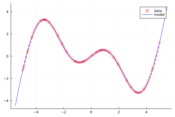
We use HaltonSampling to sample 150 data points from the input variable, evaluate the model, and fit a LinearBasisFunctionModel using a MonomialBasis of degree $d=9$.

x = RandomVariable(Uniform(-5, 5), :x)
y = Model(
        df -> df.x .* cos.(df.x),
        :y,
    )
data = sample(x, HaltonSampling(150))
evaluate!(y, data)
lbfm = LinearBasisFunctionModel(data, :y, MonomialBasis(1, 9))

ResponseSurface(MonomialBasis(1, 9, Monomials.Monomial[1, x1, x1², x1³, x1⁴, x1⁵, x1⁶, x1⁷, x1⁸, x1⁹]), [0.00018241593646902075, 0.9878644609495059, -0.00018150970456987044, -0.48925985169682223, 4.747249404303626e-5, 0.038987490233917725, -3.913393749589379e-6, -0.0011115728398402001, 9.668870671278248e-8, 1.1603496934147144e-5], [:x], :y)

A plot comparing the resulting model to the data points is presented next.

Response Surface

A linear basis function model constructed from a MonomialBasis is also known as a polynomial Response Surface [ DocumenterCitations.CitationSiteNode("khuriResponseSurfaceMethodology2010-cite-1")

]. For this reason we provide a convenient alias ResponseSurface. Using this alias the previous example can be adapted as follows.

rs = ResponseSurface(data, :y, 9)

ResponseSurface(MonomialBasis(1, 9, Monomials.Monomial[1, x1, x1², x1³, x1⁴, x1⁵, x1⁶, x1⁷, x1⁸, x1⁹]), [0.00018241593646902075, 0.9878644609495059, -0.00018150970456987044, -0.48925985169682223, 4.747249404303626e-5, 0.038987490233917725, -3.913393749589379e-6, -0.0011115728398402001, 9.668870671278248e-8, 1.1603496934147144e-5], [:x], :y)

Design Of Experiments

Several experimental designs have been developed to efficiently estimate ResponseSurface models [ DocumenterCitations.CitationSiteNode("khuriResponseSurfaceMethodology2010-cite-2")

]. Although designed for response surface methodology these designs can be used to fit any metamodel. However, for more complex models we suggest using Quasi Monte Carlo sampling schemes instead.

The designs implemented in UncertaintyQuantification are TwoLevelFactorial, FullFactorial, FractionalFactorial, CentralComposite, BoxBehnken, and PlackettBurman.

Interval Predictor Model

An interval predictor model (IPM)[ DocumenterCitations.CitationSiteNode("crespoIntervalPredictorModels2016-cite-1")

] is a function that returns an interval instead of a precise value for the dependent variable given as

$$I_y(x,P)=\{y=p^T\phi (x),p\in P\},$$

where $\phi (x)$ is an arbitrary basis and the uncertainty set $P$ is defined as

$$P=\{p:\underset{―}{p}\le p\le \bar{p}\}.$$

Using the defining vertices of P $\underset{―}{p}$ and $\bar{p}$ the IPM results as

$$I_y(x,P)=[\underset{―}{y}(x,\bar{p},\underset{―}{p}),\bar{y}(x,\bar{p},\underset{―}{p})],$$

with

$$\underset{―}{y}(x,\bar{p},\underset{―}{p})={\bar{p}}^T\left(\frac{\phi (x)-|\phi (x)|}{2}\right)+{\underset{―}{p}}^T\left(\frac{\phi (x)+|\phi (x)|}{2}\right)$$

and

$$\bar{y}(x,\bar{p},\underset{―}{p})={\bar{p}}^T\left(\frac{\phi (x)+|\phi (x)|}{2}\right)+{\underset{―}{p}}^T\left(\frac{\phi (x)-|\phi (x)|}{2}\right).$$

Here, $\underset{―}{y}$ and $\bar{y}$ are the lower and upper bounds of the IPM.

The distance between the lower and upper bound given by

$${\delta }_y(x,\bar{p},\underset{―}{p})=(\bar{p}-\underset{―}{p}{)}^T|\phi (x)|$$

is known as the spread of the IPM. The optimal defining vertices for a given data set are found by minimizing the average spread such that all data points fall into the IPM by solving the following convex constrained optimization problem.

$$\{\underset{―}{p},\bar{p}\}=\underset{u,v}{\mathrm{argmax}}\{{\mathbb{E}}_x[{\delta }_y(x,u,v]:\underset{―}{y}(x_i,v,u)\le y_i\le \bar{y}(x_i,v,u),u\le v\}$$

Example

Consider the function

$$y(x)=x^2\cos (x)-\sin (3x)\exp (-x^2)-x-\cos (x^2)+xg,$$

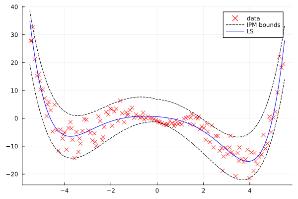
where $x\sim U(-5.5,5.5$ and $g\sim N(0,1)$. We generate a data sequence of $N=150$ points and fit an IntervalPredictorModel using a MonomialBasis of sixth degree.

x = RandomVariable(Uniform(-5.5, 5.5), :x)
data = sample(x, HaltonSampling(150))

m = Model(
        df ->
            df.x .^ 2 .* cos.(df.x) .- sin.(3 * df.x) .* exp.(-df.x .^ 2) .- df.x .-
            cos.(df.x .^ 2) .+ df.x .* randn(size(df, 1)),
        :y,
    )

evaluate!(m, data)

b = MonomialBasis(1,6)
ipm = IntervalPredictorModel(data, :y, b)

IntervalPredictorModel{MonomialBasis}(MonomialBasis(1, 6, Monomials.Monomial[1, x1, x1², x1³, x1⁴, x1⁵, x1⁶]), [-1.2720546724495774, -2.547509011220345, -1.8441520363249984, 0.03628854681653243, 0.04630398819605291, -6.102061289813858e-5, 0.0013326512447875813], [6.780543527846371, -0.5173681859439141, -1.8441520363249966, 0.036288546816527135, 0.04630398819605069, -6.102061289878519e-5, 0.0013326512447874406], [:x], :y, 150)

The following figure presents the bounds of the resulting IPM and the corresponding least squares solution. Note, that the least squares solution is not guaranteed to be between the bounds of the IPM.

IPM reliability

The reliability of the IPM, that is the probability that and unobserved data point $(x,y)$ will fall in the interval $I_y(x,P)$ can be assessed using the reliability function. The function reliability(ipm, ϵ) returns the confidence parameter $\beta$. Then, the reliability of the IPM is no less than $1-ϵ$ with confidence $1-\beta$.

1 - reliability(ipm, 0.1548)

0.9898502075787752

Reliability analysis

As the IPM is an imprecise model, it can only be applied in a reliability analysis using the DoubleLoop or RandomSlicing. For more information, see Imprecise Reliability Analysis.

Gaussian Process Regression

Theoretical Background

A Gaussian Process (GP) is a collection of random variables, any finite subset of which has a joint Gaussian distribution. It is fully specified by a mean function $m(x)$ and a covariance (kernel) function $k(x,x^{\prime })$. In GP regression, we aim to model an unknown function $f(x)$. Before observing any data, we assume that the function $f(x)$ is distributed according to a GP:

$$f(x)\sim \mathcal{G}\mathcal{P}(m(x),k(x,x^{\prime })).$$

This prior GP specifies that any finite collection of function values follows a multivariate normal distribution.

To define a prior GP we use AbstractGPs.jl for the GP interface and mean function, and KernelFunctions.jl for the definition of a covariance kernel. Below, we construct a simple prior GP with a constant zero mean function and a scaled squared exponential kernel:

using UncertaintyQuantification

kernel = SqExponentialKernel() ∘ ScaleTransform(3.0)

Note that the definition of a prior GP is handled by UncertaintyQuantification if no prior GP is specified. The construction of a GaussianProcess is flexible. Mean functions, kernels and many other parameters can be specified later directly in the constructor of the GaussianProcess.

Posterior Gaussian Process

The posterior GP represents the distribution of functions after incorporating observed data. We denote the observation data as:

$$\mathcal{D}=\{({\hat{x}}_i,{\hat{f}}_i)\mid i=1,\dots ,N\},$$

where ${\hat{f}}_i=f({\hat{x}}_i)$ in the noise-free observation case, and ${\hat{f}}_i=f({\hat{x}}_i)+e_i$ in the noisy case, with independent noise terms $e_i\sim \mathcal{N}(0,{\sigma }_e^2)$. Let $\hat{X}=[{\hat{x}}_1,\dots ,{\hat{x}}_N]$ denote the collection of observation data locations. The corresponding mean vector and covariance matrix are:

$$\mu (\hat{X})=[m({\hat{x}}_1),\dots ,m({\hat{x}}_N)],K(\hat{X},\hat{X})\text{ with entries }{K}_{ij}=k({\hat{x}}_i,{\hat{x}}_j).$$

For a new input location $x^{\ast }$ we are interested at the unknown function value $f^{\ast }=f(x^{\ast })$. By the definition of a GP, the joint distribution of observed outputs ${\hat{f}}_i$ and the unknown $f^{\ast }$ is multivariate Gaussian:

$$\left[\begin{array}{c}\hat{f}\\ f^{\ast }\end{array}\right]=\mathcal{N}(\left[\begin{array}{c}\mu (\hat{X})\\ m(x^{\ast })\end{array}\right],\left[\begin{array}{cc}K(\hat{X},\hat{X})& K(\hat{X},x^{\ast })\\ K(x^{\ast },\hat{X})& K(x^{\ast },x^{\ast })\end{array}\right]),$$

where:

• $K(\hat{X},\hat{X})$ is the covariance matrix with entries $K_{ij}=k({\hat{x}}_i,{\hat{x}}_j)$,

• $K(\hat{X},x^{\ast })$ is the covariance matrix with entries $K_{i1}=k({\hat{x}}_i,x^{\ast })$,

• and $(x^{\ast },x^{\ast })$ is the variance at the unknown input location.

We can then obtain the posterior distribution of $f^{\ast }$ from the properties of multivariate Gaussian distributions (see, e.g. Appendix A.2 in [ DocumenterCitations.CitationSiteNode("rasmussen2005gaussian-cite-1")

]), by conditioning the joint Gaussian on the observed outputs ${\hat{f}}_i$:

$$f^{\ast }\mid \hat{X},\hat{f},x^{\ast }\sim \mathcal{N}({\mu }^{\ast }(x^{\ast }),{\mathrm{\Sigma }}^{\ast }(x^{\ast })),$$

with

$$\begin{gathered} {\mu }^{\ast }(x^{\ast })=m(x^{\ast })+K(x^{\ast },\hat{X})K(\hat{X},\hat{X}{)}^{-1}(\hat{f}-\mu (\hat{X})), \\ {\mathrm{\Sigma }}^{\ast }(x^{\ast })=K(x^{\ast },x^{\ast })-K(x^{\ast },\hat{X})K(\hat{X},\hat{X}{)}^{-1}K(\hat{X},x^{\ast }). \end{gathered}$$

In the noisy observation case, the covariance between training points is adjusted by adding the noise variance:

$$K(\hat{X},\hat{X})\to K(\hat{X},\hat{X})+{\sigma }_e^{2}I.$$

The computation of the posterior predictive distribution generalizes straightforwardly to multiple input locations, providing both the posterior mean, which can serve as a regression estimate of the unknown function, and the posterior variances, which quantify the uncertainty at each point. Because the posterior is multivariate Gaussian, one can also sample function realizations at specified locations to visualize possible functions consistent with the observed data.

To construct a posterior GP, we need to define training data in form of a DataFrame. Constructing a GaussianProcess model will then automatically compute the posterior GP to predict requested the modeled output $y$ and by default it will also optimize the hyperparameters. If this is not desired, the input learn_hyperparameters=false can be set.

The following creates a standard GP with mean function ConstMean(), kernel SqExponentialKernel(), and directly optimizes the hyperparameters. Note that while ConstMean(0.0) and ZeroMean() provide the same zero-mean prior GP, using ConstMean() also allows for optimization of the mean. We also equip the GP with small observation noise ${\sigma }^2$, which has implications on the numerical stability and allows the GP to handle imprecise data. The noise can also be optimized as part of the hyperparameter optimization, but it is not optimized by default. To specify different mean functions and/or kernels, either construct a GP manually beforehand, or use them as inputs.

x = collect(range(0, 10, 10))
y = sin.(x) + 0.3 * cos.(2 .* x)
df = DataFrame(x = x, y = y)

mean_fct = ConstMean(0.0)
kernel = SqExponentialKernel() ∘ ScaleTransform(3.0)

gp_prior = GP(mean_fct, kernel)

σ² = 1e-5

# these are equivalent
gp_model = GaussianProcess(gp_prior, df, :y; σ²=σ²)
gp_model = GaussianProcess(df, :y; σ²=σ², mean_fct=mean_fct, kernel=kernel)
# providing the input learn_noise=true also optimizes the data noise

Now we can use our GP model to predict at new input locations x_test:

x_test = collect(range(0, 5, 500))
prediction = DataFrame(:x => x_test)

evaluate!(gp_model, prediction; mode=:mean_and_var)


plot!(
    x_test, prediction_mean, ribbon=2 .* prediction_std,
    color=:grey, alpha=0.5, label="Confidence band"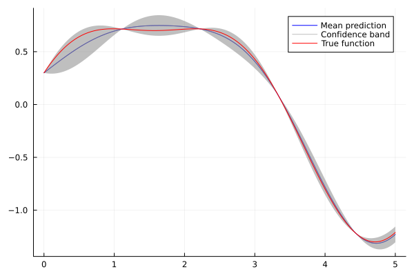

Hyperparameter optimization

GP models typically contain hyperparameters in their mean functions $m(x;{\theta }_m)$ and covariance kernel functions $k(x,x^{\prime };{\theta }_k)$. The observation noise variance ${\sigma }_e^2$ is also considered a hyperparameter related to the kernel. The choice of hyperparameters strongly affects the quality of the posterior GP.

A common approach to selecting hyperparameters is maximum likelihood estimation (MLE) (see, e.g. [ DocumenterCitations.CitationSiteNode("rasmussen2005gaussian-cite-2")

]), where we maximize the likelihood of observing the training data $\mathcal{D}$ under the chosen GP prior.

The marginal likelihood of the observed training outputs $\hat{f}$ is:

$$p(\hat{f}\mid \hat{X},{\theta }_m,{\theta }_k,{\sigma }_e^2)=\mathcal{N}(\hat{f}\mid {\mu }_{{\theta }_m}(\hat{X}),K_{{\theta }_k}(\hat{X},\hat{X})+{\sigma }_e^{2}I),$$

where ${\mu }_{{\theta }_m}(\hat{X})$ and $K_{{\theta }_k}(\hat{X},\hat{X})$ denote the parameter dependent versions of the previously defined quantities.

For numerical reasons, the logarithm of the marginal likelihood is typically used. Maximizing the log marginal likelihood with respect to the hyperparameters then yields the parameters that best explain the observed data. After obtaining the optimal hyperparameters, the posterior GP can be constructed as described above.

UncertaintyQuantification.jl provides a default optimizer for the hyperparameters based on the MaximumLikelihoodEstimation constructor.

optimizer::AbstractHyperparameterOptimization=MaximumLikelihoodEstimation(Optim.LBFGS(), Optim.Options(; iterations=100, show_trace=false))

If other options are desired, a different optimizer can be constructed based on Optim.jl. The script below shows the difference between an optimized and unoptimized GP.

using Optim

optimization = MaximumLikelihoodEstimation(
                Optim.LBFGS(),
                Optim.Options(; iterations=10, show_trace=false)
            )

gp_model = GaussianProcess(df, :y;
                           σ²=σ²,
                           mean_fct=mean_fct,
                           kernel=kernel,
                           optimizer=optimization
                           )

gp_model_unoptimized = GaussianProcess(df, :y;
                            σ²=σ²,
                            mean_fct=mean_fct,
                            kernel=kernel,
                            learn_hyperparameters=false
                           )

prediction = DataFrame(:x => x_test)
prediction_unopt = DataFrame(:x => x_test)
evaluate!(gp_model, prediction; mode=:mean_and_var)
evaluate!(gp_model_unoptimized, prediction_unopt; mode=:mean_and_var)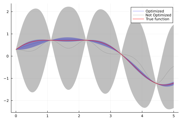

Internally, MaximumLikelihoodEstimation() defaults to using LBFGS optimizer that performs 100 optimization steps with standard optimization hyperparameters as defined Optim.jl. Note that any other first-order optimizer supported by Optim.jl, along with its corresponding hyperparameters, can also be used when constructing MaximumLikelihoodEstimation.

During optimization, GP hyperparameters ${\theta }_m,{\theta }_k$ and ${\sigma }_e^2$ are automatically extracted and updated.

We support the automatic extraction of hyperparameters from mean functions provided by AbstractGPs.jl, with the exception of:

• Custom mean functions CustomMean. These are defined with a custom function that itself could depend on hyperparameters. These additional hyperparameters are ignored in the optimization.

Kernel functions are defined with the kernels and transformations provided by KernelFunctions.jl. For similar reasons as with CustomMean, we do not extract potential function hyperparameters from the following kernels or transforms:

• Transforms defined with custom functions FunctionTransform,

• The GibbsKernel, which models a kernel lengthscale parameter with the help of a function.

Further, GP models containing the following kernels are not supported for hyperparameter optimization currently:

• Multi-output kernels MOKernel,

• Neural kernel networks [NeuralKernelNetwork].

Adaptive Gaussian Process Regression

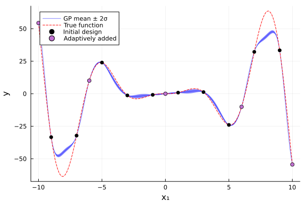
Fitting a good GP surrogate can require many expensive model evaluations if the initial experimental design is chosen naively. Adaptive (or active learning) Gaussian process regression instead starts from a small initial design and iteratively enriches the training data: at each iteration a set of candidate points is sampled from the input space, an acquisition function (also called a learning function) scores every candidate, the most promising candidate is evaluated with the true (expensive) model, and the GP is refitted with the enlarged training set. This is repeated for a fixed number of iterations, or until the acquisition function's own convergence criterion is met.

The AdaptiveGaussianProcess function drives this loop. It first constructs (or accepts) an initial GaussianProcess, then calls evaluate! on the supplied model for each newly selected point.

x = RandomVariable(Uniform(-10, 10), :x1)
model = Model(df -> sin.(df.x1) .* df.x1 .^ 2, :y)

mean_f = ConstMean(0.0)
kernel = Matern52Kernel()
gp_prior = GP(mean_f, kernel)

n_design_points = 10
n_added_points = 5

adaptive_gp = AdaptiveGaussianProcess(
    gp_prior,
    x,
    model,
    :y,
    MaximumVariance(),
    n_added_points,
    n_design_points,
)

As with GaussianProcess, the initial n_design_points are sampled with an experimental_design (LatinHypercubeSampling by default), while the n_added_points adaptively selected candidates are drawn from candidate_sampling, a Monte Carlo sampling scheme (MonteCarlo(100_000) by default). Hyperparameters can be re-optimized after every added point via learn_hyperparameters (default true).

The resulting adaptive_gp is a regular GaussianProcess and can be evaluated as usual:

using DataFrames
using Plots

test_data = DataFrame(x1 = -10:0.1:10)
evaluate!(adaptive_gp, test_data; mode = :mean_and_var)
evaluate!(model, test_data)

p = plot(test_data.x1, test_data.y_mean; ribbon = 2 .* sqrt.(test_data.y_var), label = "GP mean ± 2σ", xlabel = "x₁", ylabel = "y", color = :blue, alpha = 0.5)
plot!(p, test_data.x1, test_data.y; label = "True function", color = :red, linestyle = :dash)
scatter!(p, adaptive_gp.training_data.x1[1:n_design_points], adaptive_gp.training_data.y[1:n_design_points]; label = "Initial design", color = :black)
scatter!(p, adaptive_gp.training_data.x1[(n_design_points + 1):end], adaptive_gp.training_data.y[(n_design_points + 1):end]; label = "Adaptively added")

Acquisition Functions

The acquisition function determines which candidate point is added next, and therefore what the adaptive scheme optimizes for. Given the posterior mean $\mu (\mathbf{x})$ and posterior standard deviation $\sigma (\mathbf{x})$ of the current GP, the next point ${\mathbf{x}}^{+}$ is chosen from the sampled candidates $\mathbf{x}\in {\mathcal{X}}_c$ by maximizing (or minimizing) a criterion $a(\mathbf{x})$. For a review of various acquisition functions we refer to [ DocumenterCitations.CitationSiteNode("fuhg2021state-cite-1")

].

UncertaintyQuantification.jl provides the following acquisition functions to adapatively refine GP regression models; we separate them by there main area of application:

General active learning

Goal: improve the global fit of the GP

• MaximumVariance simply adds the point of maximum posterior variance,

$${\mathbf{x}}^{+}=\underset{\mathbf{x}\in {\mathcal{X}}_c}{\mathrm{argmax}}{\sigma }^2(\mathbf{x}).$$

• MaximinDistance is a space-filling criterion that adds the candidate farthest (in input space) from every existing training point ${\hat{\mathbf{x}}}_i\in \hat{X}$,

$${\mathbf{x}}^{+}=\underset{\mathbf{x}\in {\mathcal{X}}_c}{\mathrm{argmax}}\underset{i}{min}\Vert \mathbf{x}-{\hat{\mathbf{x}}}_i\Vert .$$

• ExpectedImprovementForGlobalFit (EIGF) trades off the local discrepancy to the nearest training observation ${\hat{f}}_{i(\mathbf{x})}$ (with $i(\mathbf{x})={\mathrm{argmin}}_i\Vert \mathbf{x}-{\hat{\mathbf{x}}}_i\Vert$) against the posterior variance,

$${\mathbf{x}}^{+}=\underset{\mathbf{x}\in {\mathcal{X}}_c}{\mathrm{argmax}}{[\mu (\mathbf{x})-{\hat{f}}_{i(\mathbf{x})}]}^2+{\sigma }^2(\mathbf{x}).$$

Bayesian optimization

Goal: refine the global minimum ${\hat{f}}_{\text{best}}=\underset{i}{min}{\hat{f}}_i$

• ExpectedImprovement with exploration parameter $\xi$,

$$\mathrm{EI}(\mathbf{x})=({\hat{f}}_{\text{best}}-\mu (\mathbf{x})-\xi )\mathrm{\Phi }(z)+\sigma (\mathbf{x})\varphi (z),z=\frac{{\hat{f}}_{\text{best}}-\mu (\mathbf{x})-\xi }{\sigma (\mathbf{x})},$$$${\mathbf{x}}^{+}=\underset{\mathbf{x}\in {\mathcal{X}}_c}{\mathrm{argmax}}\mathrm{EI}(\mathbf{x}),$$

where $\mathrm{\Phi }$ and $\varphi$ are the standard normal cdf and pdf, respectively ($\mathrm{EI}(\mathbf{x})=0$ if $\sigma (\mathbf{x})=0$).

• ProbabilityOfImprovement,

$$\mathrm{PI}(\mathbf{x})=\mathrm{\Phi }(z),z=\frac{{\hat{f}}_{\text{best}}-\mu (\mathbf{x})-\xi }{\sigma (\mathbf{x})},{\mathbf{x}}^{+}=\underset{\mathbf{x}\in {\mathcal{X}}_c}{\mathrm{argmax}}\mathrm{PI}(\mathbf{x}).$$

• UpperConfidenceBound with exploration weight $\kappa$ minimizes a lower confidence bound (for a minimization objective),

$${\mathbf{x}}^{+}=\underset{\mathbf{x}\in {\mathcal{X}}_c}{\mathrm{argmin}}\mu (\mathbf{x})-\kappa \sigma (\mathbf{x}).$$

Reliability analysis

Goal: refine the limit-state surface $g(\mathbf{x})=\tau$ (typically, $\tau =0$):

• DeviationNumber, the $U$-function used in AK-MCS, adds the point closest to the limit state relative to its uncertainty,

$${\mathbf{x}}^{+}=\underset{\mathbf{x}\in {\mathcal{X}}_c}{\mathrm{argmin}}U(\mathbf{x}),U(\mathbf{x})=\frac{|\mu (\mathbf{x})-\tau |}{\sigma (\mathbf{x})}.$$

• ExpectedFeasibility (EFF) integrates the probability that the true response lies within an $ϵ$-band $ϵ(\mathbf{x})=\text{epsilon\_factor}\cdot \sigma (\mathbf{x})$ around the limit state,

$$\begin{array}{rl}\mathrm{EFF}(\mathbf{x})=& (\mu (\mathbf{x})-\tau )[2\mathrm{\Phi }(z)-\mathrm{\Phi }(z^{-})-\mathrm{\Phi }(z^{+})]\\ & -\sigma (\mathbf{x})[2\varphi (z)-\varphi (z^{-})-\varphi (z^{+})]+ϵ(\mathbf{x})[\mathrm{\Phi }(z^{+})-\mathrm{\Phi }(z^{-})],\end{array}$$$$z=\frac{\tau -\mu (\mathbf{x})}{\sigma (\mathbf{x})},z^{-}=\frac{\tau -ϵ(\mathbf{x})-\mu (\mathbf{x})}{\sigma (\mathbf{x})},z^{+}=\frac{\tau +ϵ(\mathbf{x})-\mu (\mathbf{x})}{\sigma (\mathbf{x})},$$$${\mathbf{x}}^{+}=\underset{\mathbf{x}\in {\mathcal{X}}_c}{\mathrm{argmax}}\mathrm{EFF}(\mathbf{x}).$$