Asia Bayesian Network

The Asia network [15] is the classic small Bayesian Network used to introduce probabilistic reasoning in medical diagnosis. A patient may have visited Asia (raising the chance of tuberculosis) and may smoke (raising the chance of lung cancer and bronchitis). Tuberculosis and lung cancer both manifest through a chest X-ray, while dyspnoea (shortness of breath) is driven by that same tuberculosis-or-cancer condition together with bronchitis.

Every variable is binary, so the whole model is an ordinary BayesianNetwork built from DiscreteNodes. One rule to keep in mind: EnhancedBayesianNetworks requires state names to be unique across the whole network, so instead of a bare :yes/:no on every node we prefix each state with its variable (:A_yes, :T_yes, ...).

using EnhancedBayesianNetworks

The root causes

Two independent root nodes: a recent visit to Asia, and whether the patient smokes.

A = DiscreteNode(:A)                 # visit to Asia
A[:A => :A_yes] = 0.01
A[:A => :A_no] = 0.99

S = DiscreteNode(:S)                 # smoker
S[:S => :S_yes] = 0.5
S[:S => :S_no] = 0.5

0.5

The diseases

Tuberculosis depends on the visit to Asia; lung cancer and bronchitis depend on smoking.

T = DiscreteNode(:T, [:A])           # tuberculosis
T[:A => :A_yes, :T => :T_yes] = 0.05
T[:A => :A_yes, :T => :T_no] = 0.95
T[:A => :A_no, :T => :T_yes] = 0.01
T[:A => :A_no, :T => :T_no] = 0.99

L = DiscreteNode(:L, [:S])           # lung cancer
L[:S => :S_yes, :L => :L_yes] = 0.1
L[:S => :S_yes, :L => :L_no] = 0.9
L[:S => :S_no, :L => :L_yes] = 0.01
L[:S => :S_no, :L => :L_no] = 0.99

B = DiscreteNode(:B, [:S])           # bronchitis
B[:S => :S_yes, :B => :B_yes] = 0.6
B[:S => :S_yes, :B => :B_no] = 0.4
B[:S => :S_no, :B => :B_yes] = 0.3
B[:S => :S_no, :B => :B_no] = 0.7

0.7

The logical "either" node

E encodes tuberculosis or lung cancer. It is a deterministic OR of T and L, expressed as a CPT whose entries are just 0 and 1.

E = DiscreteNode(:E, [:T, :L])       # tuberculosis OR lung cancer
E[:T => :T_yes, :L => :L_yes, :E => :E_yes] = 1.0
E[:T => :T_yes, :L => :L_yes, :E => :E_no] = 0.0
E[:T => :T_yes, :L => :L_no, :E => :E_yes] = 1.0
E[:T => :T_yes, :L => :L_no, :E => :E_no] = 0.0
E[:T => :T_no, :L => :L_yes, :E => :E_yes] = 1.0
E[:T => :T_no, :L => :L_yes, :E => :E_no] = 0.0
E[:T => :T_no, :L => :L_no, :E => :E_yes] = 0.0
E[:T => :T_no, :L => :L_no, :E => :E_no] = 1.0

1.0

The observations

A chest X-ray reflects the E condition; dyspnoea depends on both E and bronchitis.

X = DiscreteNode(:X, [:E])           # positive X-ray
X[:E => :E_yes, :X => :X_yes] = 0.98
X[:E => :E_yes, :X => :X_no] = 0.02
X[:E => :E_no, :X => :X_yes] = 0.05
X[:E => :E_no, :X => :X_no] = 0.95

D = DiscreteNode(:D, [:E, :B])       # dyspnoea
D[:E => :E_yes, :B => :B_yes, :D => :D_yes] = 0.9
D[:E => :E_yes, :B => :B_yes, :D => :D_no] = 0.1
D[:E => :E_yes, :B => :B_no, :D => :D_yes] = 0.7
D[:E => :E_yes, :B => :B_no, :D => :D_no] = 0.3
D[:E => :E_no, :B => :B_yes, :D => :D_yes] = 0.8
D[:E => :E_no, :B => :B_yes, :D => :D_no] = 0.2
D[:E => :E_no, :B => :B_no, :D => :D_yes] = 0.1
D[:E => :E_no, :B => :B_no, :D => :D_no] = 0.9

0.9

Wiring the network

Assemble the nodes, connect each parent to its children with add_child!, and finalize the topology with order!.

bn = BayesianNetwork([A, S, T, L, B, E, X, D])
add_child!(bn, :A, :T)
add_child!(bn, :S, :L)
add_child!(bn, :S, :B)
add_child!(bn, :T, :E)
add_child!(bn, :L, :E)
add_child!(bn, :E, :X)
add_child!(bn, :E, :D)
add_child!(bn, :B, :D)
order!(bn)

The layered layout makes the causal flow easy to read, root causes on top, observations at the bottom.

gplot(bn, background_color = "white", legend = true, label_size = 10, node_scale = 0.8, legend_x = 5.5, legend_y = 1)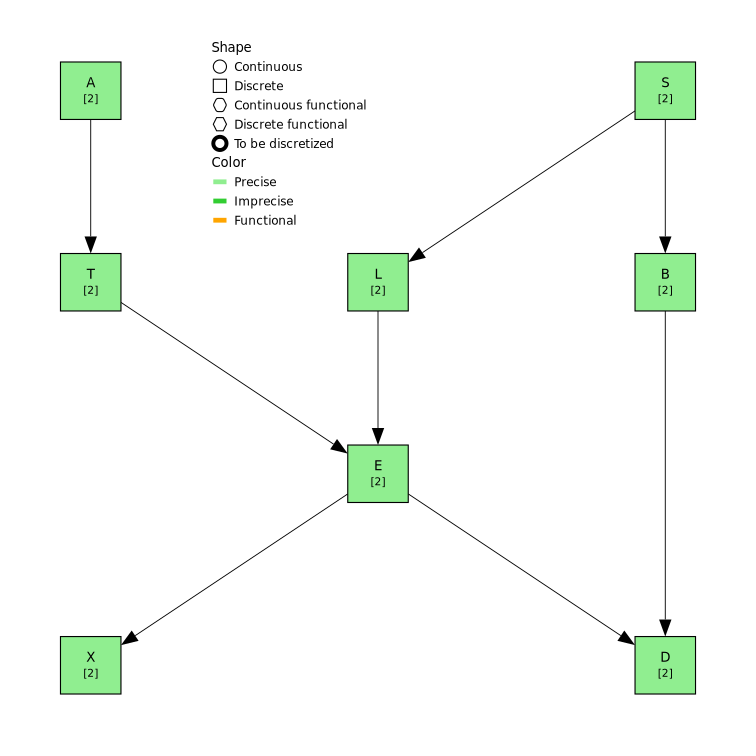

Inference

Without evidence, infer returns the prior marginal of dyspnoea.

infer(bn, :D, Evidence())

Posterior P(D)

D	Probability
------------------------
D_yes	0.43597059999999993
D_no	0.5640294

Now condition on a patient who both visited Asia and smokes, the posterior probability of dyspnoea rises accordingly.

infer(bn, :D, Evidence(:A => :A_yes, :S => :S_yes))

Posterior P(D | A=A_yes, S=S_yes)

D	Probability
------------------------
D_yes	0.5634999999999999
D_no	0.4365

We can just as well reason backwards: given a positive X-ray, how likely is lung cancer?

infer(bn, :L, Evidence(:X => :X_yes))

Posterior P(L | X=X_yes)

L	Probability
------------------------
L_yes	0.4887114013196477
L_no	0.5112885986803523

Validation against bnlearn

The Asia network ships with the bnlearn R package [16] using the identical structure and conditional probability tables. The posteriors computed above reproduce its exact (junction-tree) inference to machine precision (all values agree to ~15 significant figures), namely P(D) ≈ 0.436, P(D | asia, smoke) ≈ 0.563, and P(L | xray) ≈ 0.489. This confirms that the inference in EnhancedBayesianNetworks agrees with an established reference implementation.

Timing

As a rough indication, the wall-clock time to answer one query after compilation — measured on the machine building these docs, so treat it as indicative rather than a controlled benchmark:

infer(bn, :D, Evidence(:A => :A_yes, :S => :S_yes))   # warm up (trigger compilation)
elapsed = @elapsed infer(bn, :D, Evidence(:A => :A_yes, :S => :S_yes))
println("query solved in ", round(elapsed * 1.0e3; digits = 3), " ms")

query solved in 0.467 ms

---

This page was generated using Literate.jl.