Utility Functions

A short tour of the structural and query helpers a network provides: the Markov blanket of a node, the joint probability of a full assignment, and drawing a sample from the network.

using EnhancedBayesianNetworks

Markov blanket

The markov_blanket of a node is the set that shields it from the rest of the network — its parents, its children, and its children's other parents (co-parents). Conditioned on its blanket, a node is independent of every other node. On the network below, the blanket of x6 is its parents x3, x4, its children x9, x10, and their co-parents x5, x8.

x1 = DiscreteNode(:x1); x1[:x1 => :x1y] = 0.5; x1[:x1 => :x1n] = 0.5
x2 = DiscreteNode(:x2); x2[:x2 => :x2y] = 0.5; x2[:x2 => :x2n] = 0.5
x4 = DiscreteNode(:x4); x4[:x4 => :x4y] = 0.5; x4[:x4 => :x4n] = 0.5
x8 = DiscreteNode(:x8); x8[:x8 => :x8y] = 0.5; x8[:x8 => :x8n] = 0.5

x3 = DiscreteNode(:x3, [:x1])
x3[:x1 => :x1y, :x3 => :x3y] = 0.5; x3[:x1 => :x1y, :x3 => :x3n] = 0.5
x3[:x1 => :x1n, :x3 => :x3y] = 0.5; x3[:x1 => :x1n, :x3 => :x3n] = 0.5

x5 = DiscreteNode(:x5, [:x2])
x5[:x2 => :x2y, :x5 => :x5y] = 0.5; x5[:x2 => :x2y, :x5 => :x5n] = 0.5
x5[:x2 => :x2n, :x5 => :x5y] = 0.5; x5[:x2 => :x2n, :x5 => :x5n] = 0.5

x7 = DiscreteNode(:x7, [:x4])
x7[:x4 => :x4y, :x7 => :x7y] = 0.5; x7[:x4 => :x4y, :x7 => :x7n] = 0.5
x7[:x4 => :x4n, :x7 => :x7y] = 0.5; x7[:x4 => :x4n, :x7 => :x7n] = 0.5

x11 = DiscreteNode(:x11, [:x8])
x11[:x8 => :x8y, :x11 => :x11y] = 0.5; x11[:x8 => :x8y, :x11 => :x11n] = 0.5
x11[:x8 => :x8n, :x11 => :x11y] = 0.5; x11[:x8 => :x8n, :x11 => :x11n] = 0.5

x6 = DiscreteNode(:x6, [:x3, :x4])
x6[:x3 => :x3y, :x4 => :x4y, :x6 => :x6y] = 0.5; x6[:x3 => :x3y, :x4 => :x4y, :x6 => :x6n] = 0.5
x6[:x3 => :x3y, :x4 => :x4n, :x6 => :x6y] = 0.5; x6[:x3 => :x3y, :x4 => :x4n, :x6 => :x6n] = 0.5
x6[:x3 => :x3n, :x4 => :x4y, :x6 => :x6y] = 0.5; x6[:x3 => :x3n, :x4 => :x4y, :x6 => :x6n] = 0.5
x6[:x3 => :x3n, :x4 => :x4n, :x6 => :x6y] = 0.5; x6[:x3 => :x3n, :x4 => :x4n, :x6 => :x6n] = 0.5

x9 = DiscreteNode(:x9, [:x5, :x6])
x9[:x5 => :x5y, :x6 => :x6y, :x9 => :x9y] = 0.5; x9[:x5 => :x5y, :x6 => :x6y, :x9 => :x9n] = 0.5
x9[:x5 => :x5y, :x6 => :x6n, :x9 => :x9y] = 0.5; x9[:x5 => :x5y, :x6 => :x6n, :x9 => :x9n] = 0.5
x9[:x5 => :x5n, :x6 => :x6y, :x9 => :x9y] = 0.5; x9[:x5 => :x5n, :x6 => :x6y, :x9 => :x9n] = 0.5
x9[:x5 => :x5n, :x6 => :x6n, :x9 => :x9y] = 0.5; x9[:x5 => :x5n, :x6 => :x6n, :x9 => :x9n] = 0.5

x10 = DiscreteNode(:x10, [:x8, :x6])
x10[:x8 => :x8y, :x6 => :x6y, :x10 => :x10y] = 0.5; x10[:x8 => :x8y, :x6 => :x6y, :x10 => :x10n] = 0.5
x10[:x8 => :x8y, :x6 => :x6n, :x10 => :x10y] = 0.5; x10[:x8 => :x8y, :x6 => :x6n, :x10 => :x10n] = 0.5
x10[:x8 => :x8n, :x6 => :x6y, :x10 => :x10y] = 0.5; x10[:x8 => :x8n, :x6 => :x6y, :x10 => :x10n] = 0.5
x10[:x8 => :x8n, :x6 => :x6n, :x10 => :x10y] = 0.5; x10[:x8 => :x8n, :x6 => :x6n, :x10 => :x10n] = 0.5

x12 = DiscreteNode(:x12, [:x9])
x12[:x9 => :x9y, :x12 => :x12y] = 0.5; x12[:x9 => :x9y, :x12 => :x12n] = 0.5
x12[:x9 => :x9n, :x12 => :x12y] = 0.5; x12[:x9 => :x9n, :x12 => :x12n] = 0.5

x13 = DiscreteNode(:x13, [:x10])
x13[:x10 => :x10y, :x13 => :x13y] = 0.5; x13[:x10 => :x10y, :x13 => :x13n] = 0.5
x13[:x10 => :x10n, :x13 => :x13y] = 0.5; x13[:x10 => :x10n, :x13 => :x13n] = 0.5

net = BayesianNetwork([x1, x2, x4, x8, x5, x7, x11, x3, x6, x9, x10, x12, x13])
add_child!(net, :x1, :x3)
add_child!(net, :x2, :x5)
add_child!(net, :x4, :x7)
add_child!(net, :x8, :x11)
add_child!(net, :x3, :x6)
add_child!(net, :x4, :x6)
add_child!(net, :x5, :x9)
add_child!(net, :x6, :x9)
add_child!(net, :x6, :x10)
add_child!(net, :x8, :x10)
add_child!(net, :x9, :x12)
add_child!(net, :x10, :x13)
order!(net)

gplot(net, background_color = "white", label_size = 9)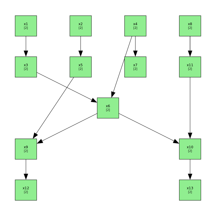

markov_blanket(net, :x6)

6-element Vector{Symbol}:
 :x5
 :x9
 :x8
 :x10
 :x4
 :x3

A fully specified sprinkler network

For the remaining helpers we use a small, completely specified BN: the weather drives whether it rains and whether the sprinkler runs, and both wet the grass.

W = DiscreteNode(:W)
W[:W => :sunny] = 0.7
W[:W => :cloudy] = 0.3

R = DiscreteNode(:R, [:W])
R[:W => :sunny, :R => :yesR] = 0.1; R[:W => :sunny, :R => :noR] = 0.9
R[:W => :cloudy, :R => :yesR] = 0.8; R[:W => :cloudy, :R => :noR] = 0.2

S = DiscreteNode(:S, [:W])
S[:W => :sunny, :S => :onS] = 0.5; S[:W => :sunny, :S => :offS] = 0.5
S[:W => :cloudy, :S => :onS] = 0.1; S[:W => :cloudy, :S => :offS] = 0.9

G = DiscreteNode(:G, [:R, :S])
G[:R => :yesR, :S => :onS, :G => :wetG] = 0.99; G[:R => :yesR, :S => :onS, :G => :dryG] = 0.01
G[:R => :yesR, :S => :offS, :G => :wetG] = 0.9; G[:R => :yesR, :S => :offS, :G => :dryG] = 0.1
G[:R => :noR, :S => :onS, :G => :wetG] = 0.9; G[:R => :noR, :S => :onS, :G => :dryG] = 0.1
G[:R => :noR, :S => :offS, :G => :wetG] = 0.0; G[:R => :noR, :S => :offS, :G => :dryG] = 1.0

bn = BayesianNetwork([W, R, S, G])
add_child!(bn, :W, :R)
add_child!(bn, :W, :S)
add_child!(bn, :R, :G)
add_child!(bn, :S, :G)
order!(bn)

gplot(bn, background_color = "white")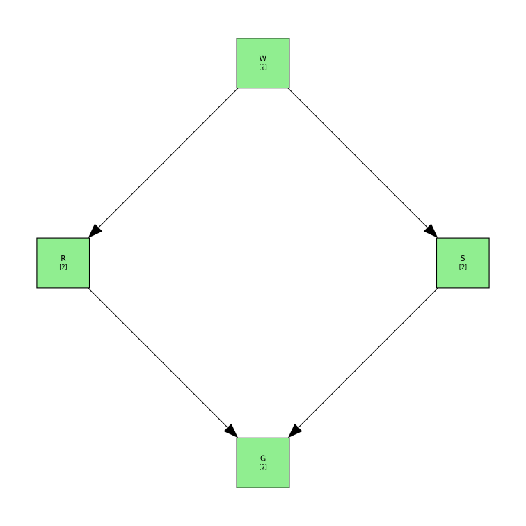

Joint probability

joint_probability evaluates the probability of a complete assignment of every node — one term of the network's factorized joint distribution. Here: a sunny day, no rain, sprinkler on, wet grass.

joint_probability(bn, Dict(:W => :sunny, :R => :noR, :S => :onS, :G => :wetG))

0.28350000000000003

Sample

sample draws one realization from the network by ancestral sampling, returning a one-row table with a state for every node.

sample(bn)

1×4 DataFrame

Row	W	R	S	G
	Symbol	Symbol	Symbol	Symbol
1	sunny	noR	onS	wetG

---

This page was generated using Literate.jl.