Plotting

gplot draws a network as a layered, top-down graph: roots on the first row, every other node one row below its deepest parent, with edges attached to the exact border of each shape. It works on any network, Bayesian Network (BN), Credal Network (CN), or Enhanced Bayesian Network (eBN), and on a DirectAcyclicGraph, so a structure can be inspected before its parameters are even learned.

W = DiscreteNode(:W)
W[:W => :sunny] = 0.7
W[:W => :rainy] = 0.3
U = ContinuousNode(:U, [:W])
U[:W => :sunny] = Normal()
U[:W => :rainy] = Normal(2, 1)
G = DiscreteNode(:G, [:W], [:yesG => [Parameter(1.0, :G)], :noG => [Parameter(0.0, :G)]])
G[:W => :sunny, :G=>:yesG] = Interval(0.4,0.6)
G[:W => :sunny, :G=>:noG] = Interval(0.4,0.6)
G[:W => :rainy, :G=>:yesG] = Interval(0.4,0.6)
G[:W => :rainy, :G=>:noG] = Interval(0.4,0.6)
model = Model(df -> df.U .* df.G, :F)
performance = df -> df.F
F = DiscreteFunctionalNode(:F, model, performance, MonteCarlo(100))

net = EnhancedBayesianNetwork([W, U, G, F])
add_child!(net, W, [U,G])
add_child!(net, [U,G], F)
order!(net)

gplot(net; title = "weather", background_color="white")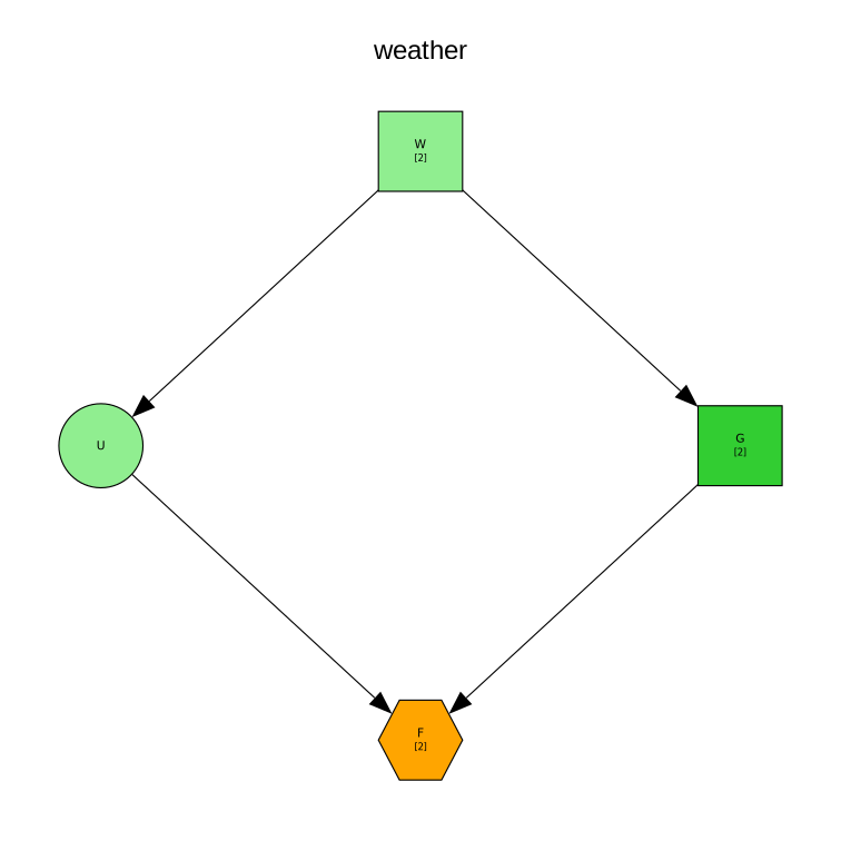

The visual language

The drawing encodes each node's kind, precision, and discretization, so the diagram doubles as a summary of the model:

Encoding	Meaning
Rectangle	discrete node
Circle	continuous node
Pointy hexagon	discrete functional node
Rounded hexagon	continuous functional node
Pale fill	precise node
Bright fill	imprecise node
Orange fill	functional node
Thick border	continuous node carrying a discretization

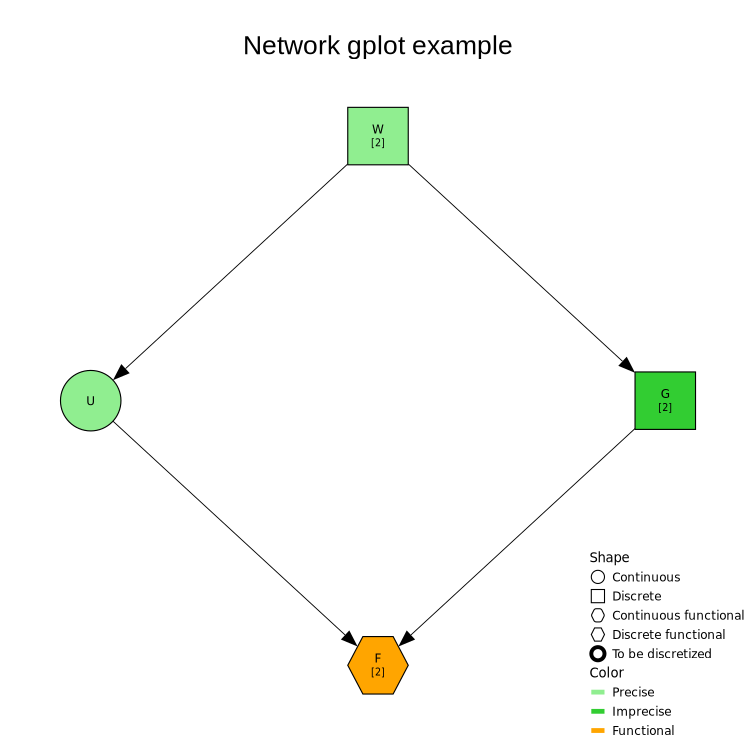
Discrete nodes also show their number of states below the name. Pass legend = true to draw the shape/colour key on the canvas (its top-left corner placed at legend_x, legend_y centimetres from the top-left of the canvas).

Customizing the drawing

gplot takes keyword arguments to size and annotate the figure:

• title, title_scale: a title above the graph and its font scale.

• node_scale: scale every node shape up or down.

• label_size: the node-label font size, in points (default 8).

• figsize: the canvas size in centimetres, a (width, height) tuple of numbers (default (20, 20)).

• background_color: the canvas background colour (default "transparent"; pass e.g. "white" for an opaque figure).

• legend: draw the shape/colour key.

• legend_x, legend_y: the legend's top-left corner, in centimetres from the top-left of the canvas (default (13, 12)).

• legend_fontsize: the legend's text size in points (default 9); the icons and spacing scale with it, so this alone sets how large the legend is.

gplot(
        net;
        node_scale        = 0.8,
        label_size        = 9,
        title             = "Network gplot example",
        title_scale       = 1.1,
        figsize           = (20, 20),
        legend            = true,
        legend_fontsize   = 9,
        legend_x          = 15.5,
        legend_y          = 14.5,
        background_color  = "white",
)

Saving to a file

gplot returns a Compose.Context. saveplot writes it to an SVG file:

p = gplot(net; title = "weather", legend = true)
saveplot(p, "weather.svg")