Nodes
Nodes are the fundamental building blocks of a Networks: together with the edges, they graphically represent the random variables of the Network. Every node carries a name (a Symbol) that uniquely identifies it, and Conditional Probability Table (CPT), which might by a priori known or unknown, and continuous or discrete. A node is classified along two independent lines.
By position in the graph a node is either a root: no parents, its state depending on nothing else. Or a child: with one or more parents that influence it. This is a property of the assembled network, read back with isroot, not a separate type.
By the nature of its variable a node is either discrete: a finite set of mutually exclusive states (discrete CPT). Or continuous: a real-valued quantity described by a probability distribution (continuous CPT).
Cutting across both is the distinction that decides which type you actually construct:
Is the node's conditional probability table (CPT) known a priori?
Yes: you supply it explicitly, as a
DiscreteNodeor aContinuousNode.No: the CPT is instead defined by a functional relationship with the parents, so the node must be functional (
DiscreteFunctionalNode,ContinuousFunctionalNode). Its table does not exist up front: it is materialized only when the enhanced Bayesian Network is reduced, by propagating the parents' uncertainty through the node's models (structural reliability problems).
| Type | Variable | CPT | Role |
|---|---|---|---|
DiscreteNode | discrete | known a priori | root or child |
ContinuousNode | continuous | known a priori | root or child |
DiscreteFunctionalNode | discrete | not known a priori | child only |
ContinuousFunctionalNode | continuous | not known a priori | child only |
The distributions, models and simulation methods a node is built from belong to UncertaintyQuantification.jl [5] and are re-exported by EnhancedBayesianNetworks, so they are available without a separate using.
CPT's entries may also be precise or imprecise: a discrete entry is a Real probability for a precise discrete node or a probability Interval for an imprecise (or credal) discrete node [7, 8]; a continuous entry is a UnivariateDistribution for a precise continuous node, while it is an Interval orProbabilityBox [3] for an imprecise continuous node [2]. Imprecision decides the resulting network type.
Among the purely discrete networks, one holding an imprecise discrete node is a Credal Network (CN) rather than a Bayesian Network (BN). An Enhanced Bayesian Network (eBN) that contains any imprecise node reduces to a CN instead of a BN.
Nodes with an a-priori-known CPT
Discrete nodes
A DiscreteNode holds a CPT over the combinations of its parents' states and its own. A root is built from its name alone; a child additionally names its parents, and every entry is filled with node[parent => state, …, name => own_state] = p. The constructor enforces that the states are mutually exclusive and collectively exhaustive.
W = DiscreteNode(:W)                        # root: CPT known a priori
W[:W => :sunny]  = 0.5
W[:W => :cloudy] = 0.5

S = DiscreteNode(:S, [:W])                  # child of W
S[:W => :sunny,  :S => :on] = 0.9
S[:W => :sunny,  :S => :off] = 0.1
S[:W => :cloudy, :S => :on] = 0.2
S[:W => :cloudy, :S => :off] = 0.8
S
DiscreteNode: S
Parents: W
States: on, off
Type: Precise
4×3 DataFrame
Row │ W S Π
│ Symbol Symbol Union…
─────┼────────────────────────
1 │ sunny on 0.9
2 │ sunny off 0.1
3 │ cloudy on 0.2
4 │ cloudy off 0.8A child's entries can be mixed across scenarios: some given as a Real probability and others as an Interval. As soon as at least one entry is an Interval, the whole node is imprecise, its CPT becomes a credal set, which calls for a CN rather than a BN:
S[:W => :sunny, :S => :on] = Interval(0.8, 0.95)
S
DiscreteNode: S
Parents: W
States: on, off
Type: Credal
4×3 DataFrame
Row │ W S Π
│ Symbol Symbol Union…
─────┼─────────────────────────────
1 │ sunny on [0.8, 0.95]
2 │ sunny off 0.1
3 │ cloudy on 0.2
4 │ cloudy off 0.8isprecise(S)falseA discrete node can also carry per-state Parameters. These are inert on their own; they matter only when the node feeds a functional node, whose models (UQModels) read them (see the functional-nodes section below):
P = DiscreteNode(:P, [:on => [Parameter(0.5, :P)], :off => [Parameter(0.0, :P)]])
P[:P => :on] = 0.7
P[:P => :off] = 0.3
P
DiscreteNode: P
Parents: none
States: on, off
Type: Precise
Parameters:
on: Parameter(0.5, :P)
off: Parameter(0.0, :P)
2×2 DataFrame
Row │ P Π
│ Symbol Union…
─────┼────────────────
1 │ on 0.7
2 │ off 0.3Continuous nodes
A ContinuousNode maps each parent-state combination to a probability distribution. A root is built directly from a single distribution; a child names its parents and assigns one distribution per parent-state combination:
T = ContinuousNode(:T, Normal())            # root from one distribution
T
ContinuousNode: T
Parents: none
Type: Precise
Support: [-Inf, Inf]
1×1 DataFrame
Row │ Π
│ Union…
─────┼───────────────────────────────
1 │ Normal{Float64}(μ=0.0, σ=1.0)isroot(T), isprecise(T)(true, true)C = ContinuousNode(:C, [:W]) # child: one distribution per parent state
C[:W => :sunny] = Normal()
C[:W => :cloudy] = Normal(2, 1)
CContinuousNode: C
Parents: W
Type: Precise
Support: [-Inf, Inf]
2×2 DataFrame
Row │ W Π
│ Symbol Union…
─────┼───────────────────────────────────────
1 │ sunny Normal{Float64}(μ=0.0, σ=1.0)
2 │ cloudy Normal{Float64}(μ=2.0, σ=1.0)scenarios(C)2-element Vector{Vector{Pair{Symbol, Symbol}}}:
[:W => :sunny]
[:W => :cloudy]A continuous entry is precise when it is a UnivariateDistribution; using an Interval or a ProbabilityBox instead represents epistemic uncertainty (i.e. imprecise entry). As with discrete nodes, a child's entries may be mixed across parent-state combinations, a UnivariateDistribution for some scenarios and an Interval` or a Probability Box for others, and a single imprecise entry makes the whole node imprecise.
Discretization
Reduction eliminates continuous nodes, so a continuous node's posterior cannot be recovered afterward. To keep evidence observable on a continuous node and to let it enter discrete inference, it can be discretized [1]: its support is partitioned at a list of interval edges into a discrete node plus a conditioned continuous remainder. The strategy is attached to the node and depends on its position:
a root carries an
ExactDiscretization: the discrete probabilities follow exactly from the node's distribution, because the marginal is known;a child carries an
ApproximatedDiscretization: the marginal is not generally available, so the tails are approximated (a uniform assumption over each bounded interval and an exponential assumption, with rateλ, over an unbounded tail).
Throughout,
Precise node
The scheme follows [1]. The conditional CDF of the continuous remainder
A discretization on a root truncates the node's own CDF
While a discretization on a child cannot use the (unknown) marginal, so each bounded interval is filled with a uniform assumption,
and an unbounded (right) tail with an exponential assumption of rate λ argument):
Tr = ContinuousNode(:Tr, Normal(), ExactDiscretization([-2.0, 0.0, 2.0])) # rootContinuousNode: Tr
Parents: none
Discretization: ExactDiscretization
Intervals: -2.0, 0.0, 2.0
Type: Precise
Support: [-Inf, Inf]
1×1 DataFrame
Row │ Π
│ Union…
─────┼───────────────────────────────
1 │ Normal{Float64}(μ=0.0, σ=1.0)# child: interval edges plus the exponential tail rate (here 1.5)
Cd = ContinuousNode(:Cd, [:W], ApproximatedDiscretization([-1.0, 0.0, 1.0], 1.5))ContinuousNode: Cd
Parents: W
Discretization: ApproximatedDiscretization
λ: 1.5
Intervals: -1.0, 0.0, 1.0
Type: Precise
0×2 DataFrame
Row │ W Π
│ Symbol Union…
─────┴────────────────Imprecise node
When the node is imprecise the same partition is used, but both the surrogate's interval probabilities and the residual are chosen to preserve the imprecision.
The probability mass of interval
while for a bare interval entry no CDF is available — only the support — so every interval receives the vacuous mass
Vacuous masses and conditioning
A node discretized from a bare interval is vacuous: masses of ProbabilityBox can narrow these mass intervals, but it avoids zero-probability extremes only when the lower mass of the observed bin is strictly positive.
The residual then differs by position. On a root it keeps the imprecision: a probability box is restricted to
The asymmetry is deliberate: on a root the imprecision lives in both the surrogate probabilities and the residual; on a child it is pushed entirely into the surrogate's interval probabilities, leaving a precise residual.
# imprecise root: an interval distribution, discretized exactly
Ti = ContinuousNode(:Ti, Interval(-2.0, 2.0), ExactDiscretization([-2.0, 0.0, 2.0]))
ContinuousNode: Ti
Parents: none
Discretization: ExactDiscretization
Intervals: -2.0, 0.0, 2.0
Type: Imprecise
Support: [-2.0, 2.0]
1×1 DataFrame
Row │ Π
│ Union…
─────┼─────────────
1 │ [-2.0, 2.0]# imprecise child: an interval entry plus the exponential tail rate
Ci = ContinuousNode(:Ci, [:W], ApproximatedDiscretization([-1.0, 0.0, 1.0], 1.5))
Ci[:W => :sunny] = Interval(-1.0, 1.0)
CiContinuousNode: Ci
Parents: W
Discretization: ApproximatedDiscretization
λ: 1.5
Intervals: -1.0, 0.0, 1.0
Type: Imprecise
Support: [-1.0, 1.0]
1×2 DataFrame
Row │ W Π
│ Symbol Union…
─────┼─────────────────────
1 │ sunny [-1.0, 1.0]Nodes with an a-priori-unknown CPT (functional nodes)
When a node's CPT is not known a priori, it is defined by a functional relationship with its parents: one or more UQModel, plus a simulation that propagates the parents' uncertainty through them. Models range from simple analytical expression to ExternalModel wrapping any external solver, and among the simulation techniques we have standard MonteCarlo, FORM, advanced Monte Carlo (e.g. LineSampling, ImportantSampling, SubSetSimulation), DoubleLoop and RandomSlicing. For a full description of each, see the UncertaintyQuantification.jl manual.
The resulting table is a collection of structural reliability problems, evaluated only when the network is reduced (see Reduction & Structural Reliability Problem). A functional node is therefore always a child, and never a root.
Discrete Functional nodes
A DiscreteFunctionalNode derives two states: :<name>_safe and :<name>_failed. A performance function maps the models' output to a limit state (failed where performance < 0), and the evaluated CPT stores the estimated failure probability against :<name>_failed and its complement against :<name>_safe:
model = Model(df -> df.x .^ 2, :y)          # y is computed from parent x
performance = df -> df.y .- 1.0             # failed when y < 1

DF = DiscreteFunctionalNode(:DF, [model], performance, MonteCarlo(1000))
DiscreteFunctionalNode: DF
States: DF_safe, DF_failed
Models: 1
Names: y
Simulation: MonteCarlostates(DF) # [:DF_safe, :DF_failed]2-element Vector{Symbol}:
:DF_safe
:DF_failedContinuous Functional nodes
A ContinuousFunctionalNode has no performance function: after evaluation, its model output samples are fitted into an EmpiricalDistribution, one per scenario of its discrete ancestors.
model = Model(df -> df.x .^ 2, :y)
CF = ContinuousFunctionalNode(:CF, [model], MonteCarlo(1000))
ContinuousFunctionalNode: CF
Models: 1
Names: y
Bins: 0
Simulation: MonteCarloImprecise parents give a distribution-free p-box
When a continuous functional node is fed by an imprecise continuous parent, its fitted CPT is a distribution-free (non-parametric) probability box rather than an ordinary EmpiricalDistribution. That representation is not yet available as a dedicated type — it is planned for UncertaintyQuantification.jl — so for now such a node cannot be discretized.
One simulation, or one per scenario
Passing a single simulation, e.g MonteCarlo(1000) above, reuses it for every scenario of the node's discrete ancestors. To tune the effort, or even the method, per scenario, list the parents explicitly in the constructor and then assign a simulation to each scenario the same way you would fill a CPT:
DF = DiscreteFunctionalNode(:DF, [:a, :b], [model], performance)   # list the parents
DF[:a => :a1, :b => :b1] = MonteCarlo(1000)
DF[:a => :a1, :b => :b2] = SubSetSimulation(500, 0.1, 10, Uniform(-0.2, 0.2))
DF[:a => :a2, :b => :b1] = MonteCarlo(200)
DF[:a => :a2, :b => :b2] = MonteCarlo(200)
DF
DiscreteFunctionalNode: DF
States: DF_safe, DF_failed
Models: 1
Names: y
Simulation: ScenariosTable
4×3 DataFrame
Row │ a b sim
│ Symbol Symbol Union…
─────┼───────────────────────────────────────────────────
1 │ a1 b1 MonteCarlo(1000)
2 │ a1 b2 SubSetSimulation(500, 0.1, 10, U…
3 │ a2 b1 MonteCarlo(200)
4 │ a2 b2 MonteCarlo(200)Different scenarios may use entirely different techniques (standard MonteCarlo, SubSetSimulation, a DoubleLoop, RandomSlicing or others). The same per-scenario form is available for ContinuousFunctionalNode via its ContinuousFunctionalNode(name, parents, models) constructor.
Constructing a functional node only records its models and simulation, no sampling runs until reduction, which is why states(DF) above returns immediately. Like any discrete node, a DiscreteFunctionalNode may carry parameters for when it in turn feeds a further functional node.
Imprecise parents
A functional node with only precise parents can use any single-loop simulation (FORM, Monte Carlo, Advanced Monte Carlo). If any parent is imprecise, the analysis needs a double-loop simulation (Double Loop or Random Slicing) and the reduced network becomes a CN.
Inspecting nodes
The same accessors work across node types:
states: the discrete states a node can take.scenarios: each CPT row asparent => statepairs.parents: the node's parent names (empty for a root).isroot: whether the node has no parents.isprecise: whether every entry is precise.sample: draw a state from a precise discrete node given evidence.
(states = states(W), parents = parents(S), root = isroot(W))(states = [:sunny, :cloudy], parents = [:W], root = true)Sampling draws a state consistent with fixed parent evidence (precise nodes only):
S = DiscreteNode(:S, [:W])                  # child of W
S[:W => :sunny,  :S => :on] = 0.9
S[:W => :sunny,  :S => :off] = 0.1
S[:W => :cloudy, :S => :on] = 0.2
S[:W => :cloudy, :S => :off] = 0.8
sample(S, Evidence(:W => :sunny))           # e.g. :on
:on