One-Bay Elasto-Plastic Frame

The enhanced Bayesian Network (eBN) framework of Straub & Der Kiureghian [1] couples a Bayesian Network with structural reliability methods, so that continuous random variables and physical models can live alongside ordinary discrete nodes. This example reproduces the one-bay, one-storey elasto-plastic frame from their companion application paper [18] — a classic reliability benchmark — and shows how EnhancedBayesianNetworks turns it into a plain BayesianNetwork with reduce.

The frame carries a horizontal load H and a vertical load V, and can collapse through any of three plastic mechanisms. Its resistance is governed by five plastic moment capacities at the critical sections, all lognormal and mutually correlated through a shared standard-normal factor Uᵣ.

using EnhancedBayesianNetworks

The applied loads

The two loads are continuous root nodes: a Gamma-distributed vertical load and a Gumbel-distributed horizontal load, each specified through its mean and coefficient of variation.

μ_gamma = 60         # kN  (mean vertical load V)
cov_gamma = 0.2
α, θ = distribution_parameters(μ_gamma, μ_gamma * cov_gamma, Gamma)
V = ContinuousNode(:V, Gamma(α, θ))

μ_gumbel = 50        # kN  (mean horizontal load H)
cov_gumbel = 0.4
μ_loc, β = distribution_parameters(μ_gumbel, cov_gumbel * μ_gumbel, Gumbel)
H = ContinuousNode(:H, Gumbel(μ_loc, β))

ContinuousNode: H
Parents: none
Type: Precise
Support: [-Inf, Inf]

1×1 DataFrame
 Row │ Π                                 
     │ Union…                            
─────┼───────────────────────────────────
   1 │ Gumbel{Float64}(μ=40.9989, θ=15.…

Correlated plastic moment capacities

The five moment capacities are lognormal with mean 150 and coefficient of variation 0.2, and they are correlated because they all draw on a common standard-normal factor Uᵣ. Conditional on Uᵣ, each capacity is a lognormal whose log-mean is shifted by ρ·ζ·Uᵣ and whose log-standard-deviation is reduced to √(1 − ρ²)·ζ; the correlation coefficient ρ = 0.5477 gives a pairwise correlation of ρ² ≈ 0.3 between any two capacities.

function plastic_moment_capacities(uᵣ)
    ρ = 0.5477
    μ = 150          # kN·m  (mean plastic moment capacity)
    cov = 0.2
    λ, ζ = distribution_parameters(μ, μ * cov, LogNormal)
    normal_μ = λ + ρ * ζ * uᵣ
    normal_std = sqrt((1 - ρ^2) * ζ^2)
    return exp(rand(Normal(normal_μ, normal_std)))
end

model1 = Model(df -> plastic_moment_capacities.(df.Uᵣ), :r1)
model2 = Model(df -> plastic_moment_capacities.(df.Uᵣ), :r2)
model3 = Model(df -> plastic_moment_capacities.(df.Uᵣ), :r3)
model4 = Model(df -> plastic_moment_capacities.(df.Uᵣ), :r4)
model5 = Model(df -> plastic_moment_capacities.(df.Uᵣ), :r5)

Model(Main.var"Main".var"#14#15"(), :r5)

The collapse mechanisms

The frame can fail through a sway, a beam, or a combined mechanism. The limit-state function returns the smallest of the three safety margins, and the frame is failed when that minimum drops below zero — which is what the performance function encodes.

function frame_model(r1, r2, r3, r4, r5, v, h)
    # moment capacities rᵢ in kN·m, loads v, h in kN; the factor 5 is the
    # member length in m, so 5·(load [kN]) is a moment in kN·m
    g1 = r1 + r2 + r4 + r5 - 5 * h
    g2 = r2 + 2 * r3 + r4 - 5 * v
    g3 = r1 + 2 * r3 + 2 * r4 + r5 - 5 * h - 5 * v
    return minimum([g1, g2, g3])
end

model = Model(df -> frame_model.(df.r1, df.r2, df.r3, df.r4, df.r5, df.V, df.H), :G)
performance = df -> df.G

#20 (generic function with 1 method)

Building the enhanced Bayesian Network

Uᵣ feeds the five capacity nodes — each a ContinuousFunctionalNode computed from its model — and the capacities together with the two loads feed the failure node E, a DiscreteFunctionalNode built from the limit-state model and its performance function.

Uᵣ = ContinuousNode(:Uᵣ, Normal())
R1 = ContinuousFunctionalNode(:R1, [model1], MonteCarlo(1000))
R2 = ContinuousFunctionalNode(:R2, [model2], MonteCarlo(1000))
R3 = ContinuousFunctionalNode(:R3, [model3], MonteCarlo(1000))
R4 = ContinuousFunctionalNode(:R4, [model4], MonteCarlo(1000))
R5 = ContinuousFunctionalNode(:R5, [model5], MonteCarlo(1000))

simulation = MonteCarlo(10^6)
frame = DiscreteFunctionalNode(:E, [model], performance, simulation)

nodes = [Uᵣ, V, H, R1, R2, R3, R4, R5, frame]

ebn = EnhancedBayesianNetwork(nodes)
add_child!(ebn, Uᵣ, [R1, R2, R3, R4, R5])
add_child!(ebn, [R1, R2, R3, R4, R5, V, H], frame)
order!(ebn)

gplot(ebn, background_color = "white", legend = true, label_size = 10, legend_x = 15, legend_y = 14)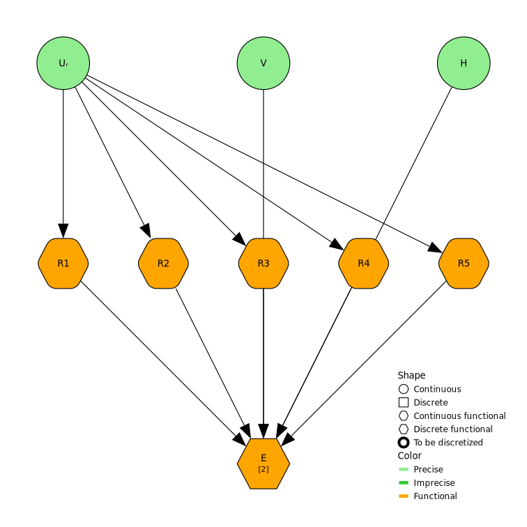

Reducing to a Bayesian Network

reduce evaluates the functional nodes in dependency order. Because none of the continuous nodes carries a discretization, the five capacity models are folded into the failure model and their continuous parents are eliminated, so the whole eBN collapses to a single discrete node whose CPT is the frame's failure probability.

bn = reduce(ebn)

BayesianNetwork

Nodes: 1
Edges: 0

Topology:

#   Node            States              Parents
--------------------------------------------------------------------------------
1   E               E_failed, E_safe    -

gplot(bn, background_color = "white", node_scale = 1.1, title = "Reduced Bayesian Network", label_size = 12)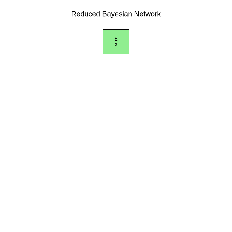

bn.nodes[1].cpt.data

2×2 DataFrame

Row	E	Π
	Symbol	Union…
1	E_failed	0.026202
2	E_safe	0.973798

Discretizing the moment capacities

The eBN framework can also retain some continuous quantities as discrete nodes in the reduced network. Attaching an ApproximatedDiscretization to R4 and R5 turns them into discrete surrogates that survive the reduction, while R1, R2 and R3 are still folded away as before.

Because EnhancedBayesianNetworks requires state names to be unique across the whole network, the two discretizations use edges offset, so R4 and R5 do not end up with identical interval labels. The edges are also chosen so that the capacities queried later (50 and 150 kNm for R4, 100 and 200 kNm for R5) fall at interval midpoints — keeping those intervals in the interior of the grid, away from the outermost bins whose edges depend on the simulated support.

discretizationr4 = ApproximatedDiscretization([20, 49, 51, 149, 151, 220], 1.5)      # edges in kN·m
discretizationr5 = ApproximatedDiscretization([20, 99, 101, 199, 201, 220], 1.5)  # edges in kN·m

Uᵣ = ContinuousNode(:Uᵣ, Normal())
R1 = ContinuousFunctionalNode(:R1, [model1], MonteCarlo(1000))
R2 = ContinuousFunctionalNode(:R2, [model2], MonteCarlo(1000))
R3 = ContinuousFunctionalNode(:R3, [model3], MonteCarlo(1000))
R4 = ContinuousFunctionalNode(:R4, [model4], MonteCarlo(1000), discretizationr4)
R5 = ContinuousFunctionalNode(:R5, [model5], MonteCarlo(1000), discretizationr5)

ContinuousFunctionalNode: R5
Models: 1
  Names: r5
Discretization: ApproximatedDiscretization
  λ: 1.5
  Intervals: 20, 99, 101, 199, 201, 220
Bins: 0
Simulation: MonteCarlo

The failure model now refers to the transferred capacities by their model output names (r1, r2, r3) and to the discretized ones by their node names (R4, R5).

simulation = MonteCarlo(10_000)
model = Model(df -> frame_model.(df.r1, df.r2, df.r3, df.R4, df.R5, df.V, df.H), :G)
frame = DiscreteFunctionalNode(:E, [model], performance, simulation)

nodes = [Uᵣ, V, H, R1, R2, R3, R4, R5, frame]

ebn = EnhancedBayesianNetwork(nodes)
add_child!(ebn, Uᵣ, [R1, R2, R3, R4, R5])
add_child!(ebn, [R1, R2, R3, R4, R5, V, H], frame)
order!(ebn)

gplot(ebn, background_color = "white", legend = true, label_size = 10, legend_x = 15, legend_y = 14)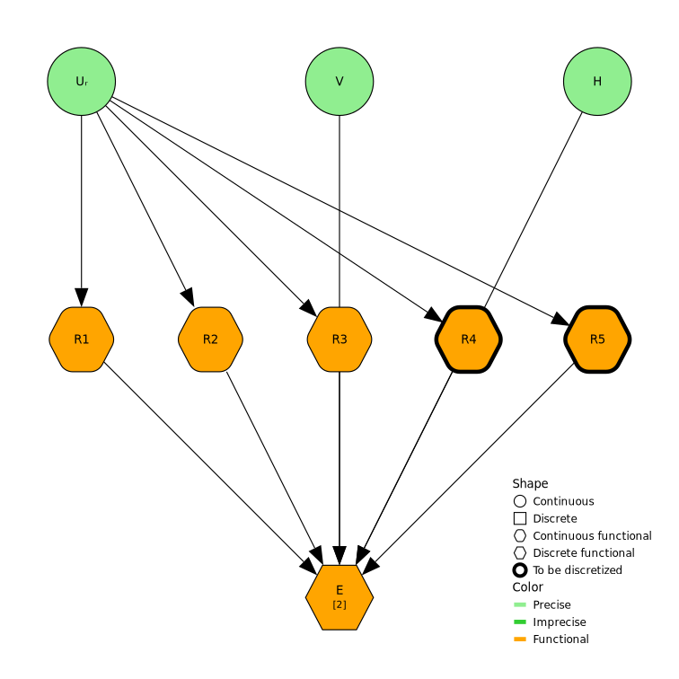

Reducing this network keeps R4 and R5 as discrete nodes — each split into a discrete surrogate and a residual continuous node — so the result is a hybrid Bayesian Network rather than a single failure node. We also time the reduction, as a rough indication measured on the machine building these docs:

elapsed = @elapsed bn = reduce(ebn)
println("network reduced in ", round(elapsed; digits = 3), " s")

┌ Warning: Node :R4 is a FunctionalNode with no discrete parents: its evaluation a single Structural Reliability Problem and its CPT will contain a single scenario.
└ @ EnhancedBayesianNetworks ~/work/EnhancedBayesianNetworks.jl/EnhancedBayesianNetworks.jl/src/networks/ebn/enhancedbn.jl:172
┌ Warning: node :R4 has minimum intervals value 20 < support lower bound 48.63999053838489. Lower bound will be used as intervals start
└ @ EnhancedBayesianNetworks ~/work/EnhancedBayesianNetworks.jl/EnhancedBayesianNetworks.jl/src/networks/ebn/discretization/discretize.jl:33
┌ Warning: node :R4 has maximum intervals value 220 < support upper bound 300.4705452050654. Upper bound will be used as intervals end
└ @ EnhancedBayesianNetworks ~/work/EnhancedBayesianNetworks.jl/EnhancedBayesianNetworks.jl/src/networks/ebn/discretization/discretize.jl:38
┌ Warning: Node :R5 is a FunctionalNode with no discrete parents: its evaluation a single Structural Reliability Problem and its CPT will contain a single scenario.
└ @ EnhancedBayesianNetworks ~/work/EnhancedBayesianNetworks.jl/EnhancedBayesianNetworks.jl/src/networks/ebn/enhancedbn.jl:172
┌ Warning: node :R5 has minimum intervals value 20 < support lower bound 36.08262812122295. Lower bound will be used as intervals start
└ @ EnhancedBayesianNetworks ~/work/EnhancedBayesianNetworks.jl/EnhancedBayesianNetworks.jl/src/networks/ebn/discretization/discretize.jl:33
┌ Warning: node :R5 has maximum intervals value 220 < support upper bound 303.8939530031974. Upper bound will be used as intervals end
└ @ EnhancedBayesianNetworks ~/work/EnhancedBayesianNetworks.jl/EnhancedBayesianNetworks.jl/src/networks/ebn/discretization/discretize.jl:38
network reduced in 10.78 s

gplot(bn, background_color = "white", node_scale = 1.1, title = "Reduced Bayesian Network", label_size = 12)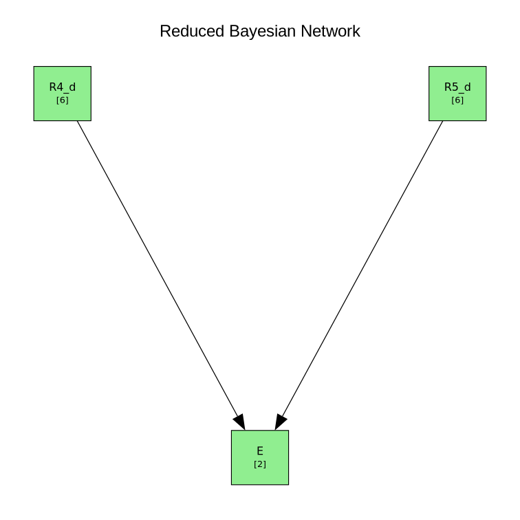

Updating the failure probability on measured capacities

With R4 and R5 now discrete, we can condition the collapse event E on observed capacity ranges — reproducing the Bayesian-updating queries of [18] (their Table 2). Each query fixes R4 and R5 to the interval centred on a measured capacity and reads off the updated probability of collapse (E_failed): a low measured capacity raises it, a high one lowers it.

First, a low capacity at section 4 (R4 ≈ 50) together with R5 ≈ 100:

e1 = Evidence(:R4_d => Symbol("[49.0, 51.0]"), :R5_d => Symbol("[99.0, 101.0]"))
infer(bn, :E, e1)

Posterior P(E | R5_d=[99.0, 101.0], R4_d=[49.0, 51.0])

E	Probability
------------------------
E_failed	0.2172
E_safe	0.7827999999999999

A higher capacity at section 4 (R4 ≈ 150), same R5 ≈ 100:

e2 = Evidence(:R4_d => Symbol("[149.0, 151.0]"), :R5_d => Symbol("[99.0, 101.0]"))
infer(bn, :E, e2)

Posterior P(E | R5_d=[99.0, 101.0], R4_d=[149.0, 151.0])

E	Probability
------------------------
E_failed	0.027
E_safe	0.973

And high capacities at both sections (R4 ≈ 150, R5 ≈ 200):

e3 = Evidence(:R4_d => Symbol("[149.0, 151.0]"), :R5_d => Symbol("[199.0, 201.0]"))
infer(bn, :E, e3)

Posterior P(E | R5_d=[199.0, 201.0], R4_d=[149.0, 151.0])

E	Probability
------------------------
E_failed	0.0102
E_safe	0.9898

The three updated collapse probabilities — roughly 0.2, 0.03 and 0.008 — are consistent with the results reported by [18] in their Table 2 (reliability indices β = 0.70, 1.80, 2.45, i.e. Pf ≈ 0.24, 0.036, 0.0071), and reproduce the same trend: the failure probability drops by roughly two orders of magnitude as the measured capacities increase. The residual differences are Monte-Carlo scatter, since the reduction estimates each conditional probability by simulation rather than the FORM used in the paper.

---

This page was generated using Literate.jl.