Parameter Learning

The networks in the other examples are written out by hand, with every conditional probability given. Often the structure is known but the numbers are not — they have to be learned from data. This example shows how EnhancedBayesianNetworks estimates the CPTs of a BayesianNetwork from a dataset: by maximum likelihood on complete data, and by expectation–maximization when some observations are missing.

To have a ground truth to compare against, we first build a fully specified network, draw synthetic data from it, and then try to recover its parameters.

using EnhancedBayesianNetworks

The reference network

The familiar sprinkler network — the weather drives whether it rains and whether the sprinkler runs, and both wet the grass. It is used only to generate data; the learning step never sees these probabilities.

W = DiscreteNode(:W)
W[:W => :sunny] = 0.7
W[:W => :cloudy] = 0.3

R = DiscreteNode(:R, [:W])
R[:W => :sunny, :R => :yesR] = 0.1
R[:W => :sunny, :R => :noR] = 0.9
R[:W => :cloudy, :R => :yesR] = 0.8
R[:W => :cloudy, :R => :noR] = 0.2

S = DiscreteNode(:S, [:W])
S[:W => :sunny, :S => :onS] = 0.5
S[:W => :sunny, :S => :offS] = 0.5
S[:W => :cloudy, :S => :onS] = 0.1
S[:W => :cloudy, :S => :offS] = 0.9

G = DiscreteNode(:G, [:R, :S])
G[:R => :yesR, :S => :onS, :G => :wetG] = 0.99
G[:R => :yesR, :S => :onS, :G => :dryG] = 0.01
G[:R => :yesR, :S => :offS, :G => :wetG] = 0.9
G[:R => :yesR, :S => :offS, :G => :dryG] = 0.1
G[:R => :noR, :S => :onS, :G => :wetG] = 0.9
G[:R => :noR, :S => :onS, :G => :dryG] = 0.1
G[:R => :noR, :S => :offS, :G => :wetG] = 0.0
G[:R => :noR, :S => :offS, :G => :dryG] = 1.0

bn = BayesianNetwork([W, R, S, G])
add_child!(bn, :W, :R)
add_child!(bn, :W, :S)
add_child!(bn, :R, :G)
add_child!(bn, :S, :G)
order!(bn)

gplot(bn, background_color = "white")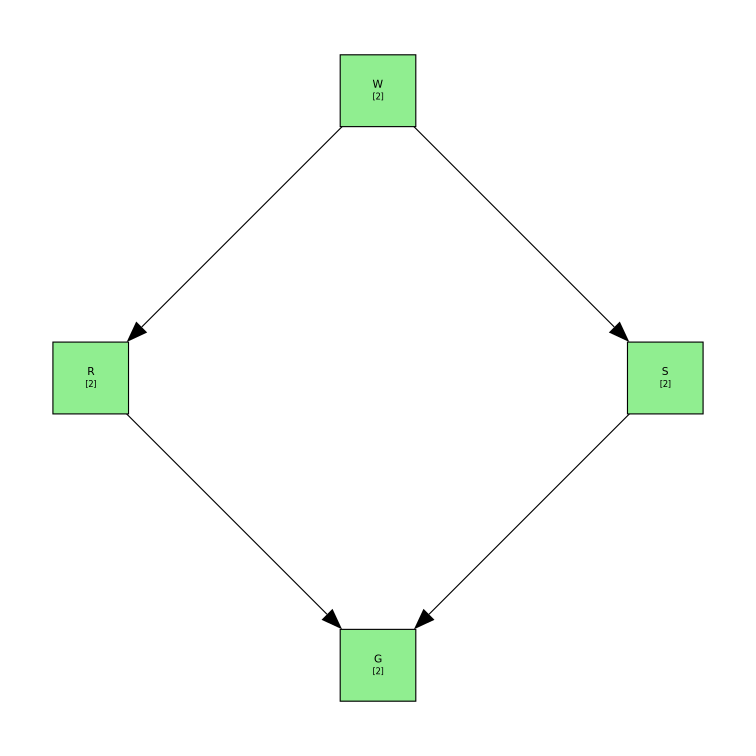

Generating a dataset

sample draws independent realizations of the whole network; a thousand rows form our observed dataset — one column per node, one row per draw (only the first ten are shown here).

df = sample(bn, 1000)
first(df, 10)

10×4 DataFrame

Row	W	R	S	G
	Symbol	Symbol	Symbol	Symbol
1	sunny	yesR	offS	wetG
2	sunny	noR	onS	wetG
3	sunny	noR	onS	wetG
4	sunny	yesR	offS	wetG
5	cloudy	yesR	offS	wetG
6	sunny	noR	onS	wetG
7	cloudy	noR	offS	dryG
8	sunny	noR	offS	dryG
9	sunny	noR	offS	dryG
10	cloudy	yesR	offS	wetG

Maximum-likelihood learning

Learning needs a structure to fill: a DirectAcyclicGraph, built node by node with add_node!, declaring each node's parents. On complete data learn estimates the CPTs by learn_parameters_mle — closed-form maximum likelihood — and the recovered probabilities closely match the network we sampled from.

dag = DirectAcyclicGraph()
add_node!(dag, :W)
add_node!(dag, :R, parents = [:W])
add_node!(dag, :S, parents = [:W])
add_node!(dag, :G, parents = [:R, :S])

learned_bn = learn(dag, df)

BayesianNetwork

Nodes: 4
Edges: 4

Topology:

#   Node            States              Parents
--------------------------------------------------------------------------------
1   W               cloudy, sunny       -
2   R               noR, yesR           W
3   S               offS, onS           W
4   G               dryG, wetG          R, S

Declaring an unobserved state

A node's states are read from the data, but extra states can be declared in add_node! even when they never occur — here a third weather state :mixed. Under plain maximum likelihood a state that was never observed gets probability zero:

dag = DirectAcyclicGraph()
add_node!(dag, :W, [:mixed])
add_node!(dag, :R, parents = [:W])
add_node!(dag, :S, parents = [:W])
add_node!(dag, :G, parents = [:R, :S])

learned_bn = learn(dag, df)
learned_bn.nodes[1]

DiscreteNode: W
Parents: none
States: cloudy, mixed, sunny
Type: Precise

3×2 DataFrame
 Row │ W       Π      
     │ Symbol  Union… 
─────┼────────────────
   1 │ cloudy  0.308
   2 │ mixed   0.0
   3 │ sunny   0.692

Smoothing with a Dirichlet prior

A Laplace/Dirichlet pseudo-count alpha adds a fictitious observation to every state, so the declared-but-unobserved :mixed receives a small non-zero probability instead of a hard zero — useful when a state is possible in principle but absent from the sample:

learned_bn = learn(dag, df, alpha = 1.0)
learned_bn.nodes[1]

DiscreteNode: W
Parents: none
States: cloudy, mixed, sunny
Type: Precise

3×2 DataFrame
 Row │ W       Π           
     │ Symbol  Union…      
─────┼─────────────────────
   1 │ cloudy  0.308076
   2 │ mixed   0.000997009
   3 │ sunny   0.690927

Incomplete data: expectation–maximization

Real datasets have gaps. Here we blank out some of the rain observations, marking them missing. When learn sees missing entries it automatically switches from the closed-form MLE to learn_parameters_em, which iteratively completes the missing values under the current estimate and re-estimates the CPTs until they converge:

df_missing = copy(df)
df_missing.R = collect(Union{Missing, Symbol}, df_missing.R)
df_missing.R[1:200] .= missing

learned_bn = learn(dag, df_missing)
learned_bn.nodes[2]

DiscreteNode: R
Parents: W
States: noR, yesR
Type: Precise

6×3 DataFrame
 Row │ W       R       Π        
     │ Symbol  Symbol  Union…   
─────┼──────────────────────────
   1 │ cloudy  noR     0.183074
   2 │ cloudy  yesR    0.816926
   3 │ mixed   noR     0.5
   4 │ mixed   yesR    0.5
   5 │ sunny   noR     0.897449
   6 │ sunny   yesR    0.102551

---

This page was generated using Literate.jl.