Imprecision on a Discrete Node

Imprecision is not confined to continuous nodes — a discrete node is imprecise whenever one of its conditional-probability entries is an interval instead of a single number. Any such node is credal, so the whole network is a CredalNetwork; the Credal Network chapter of the manual gives the full treatment.

The key point of this page: discrete imprecision never creates an imprecise continuous input, so no double loop is ever needed. Reduction and inference stay single-loop, and the surviving imprecision simply turns the result credal — lower/upper probability bounds. Two cases follow: a plain discrete network with an imprecise node, and the vehicle suspension example with an imprecise discrete node feeding a functional node.

using EnhancedBayesianNetworks

Case 1 — an imprecise discrete node, no functional node

A discrete node whose CPT carries an interval entry is imprecise; with nothing continuous or functional to reduce, the network is directly a CredalNetwork. Inference returns lower and upper probability bounds. This is the setting of the Credal Network chapter, here in miniature.

W = DiscreteNode(:W)
W[:W => :sunny] = 0.5
W[:W => :cloudy] = 0.5

S = DiscreteNode(:S, [:W])
S[:W => :sunny, :S => :on] = Interval(0.8, 0.95)   # imprecise entries
S[:W => :sunny, :S => :off] = Interval(0.05, 0.2)
S[:W => :cloudy, :S => :on] = 0.2
S[:W => :cloudy, :S => :off] = 0.8

cn = CredalNetwork([W, S])
add_child!(cn, W, S)
order!(cn)

gplot(cn, background_color = "white", legend = true, label_size = 10, legend_x = 15, legend_y = 14)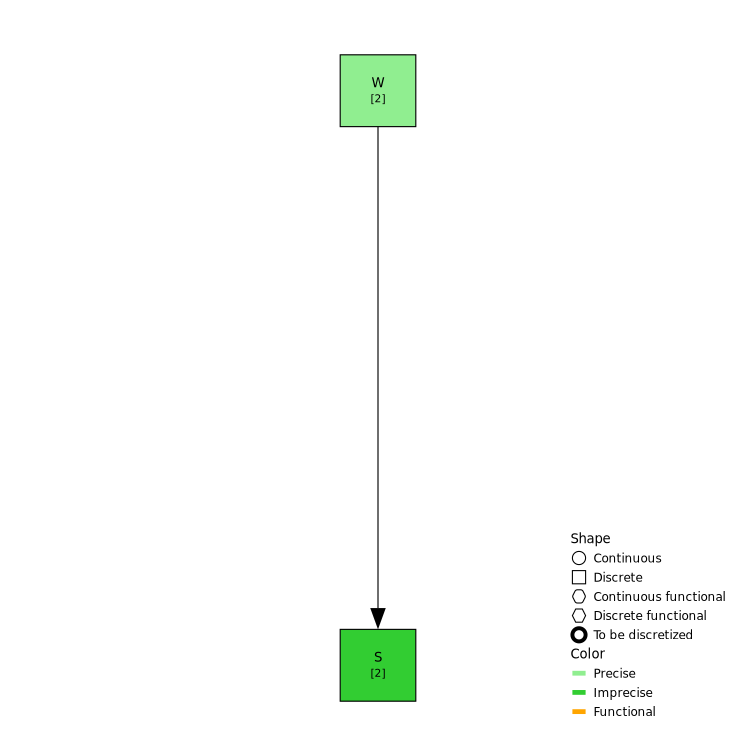

Querying S with no evidence returns a CredalPosterior — the marginal probability of each state as an interval:

infer(cn, :S, Evidence())

CredalPosterior P(S)

S	Interval
------------------------
on	[0.5, 0.575]
off	[0.425, 0.5]

Extreme posteriors: 2

Case 2 — an imprecise discrete node feeding a functional node

We reuse the vehicle suspension benchmark of Gerasimov & Vořechovský [19], but make the load coefficient b₀ imprecise: both of its states carry Interval(0.4, 0.6) probabilities. b₀ still feeds the model through its per-state Parameter values (unchanged, 0.27 and 0.5), so the structural reliability analysis at each scenario is precise and single-loop. The imprecision lives only in b₀'s credal CPT.

M = 3.2633           # kg/cm/s²  (sprung mass)
m = 0.8158           # kg/cm/s²  (unsprung mass)
g = 981              # cm/s²     (gravity)

A = DiscreteNode(:A, [:road => [Parameter(0.15915, :A)], :offroad => [Parameter(0.8, :A)]])  # A in rad·cm²/m
A[:A => :road] = 0.7
A[:A => :offroad] = 0.3

0.3

b₀ is now imprecise — an interval CPT — while its Parameter values are unchanged:

b₀ = DiscreteNode(:b₀, [:normal_load => [Parameter(0.27, :b₀)], :over_load => [Parameter(0.5, :b₀)]])
b₀[:b₀ => :normal_load] = Interval(0.4, 0.6)
b₀[:b₀ => :over_load] = Interval(0.4, 0.6)

V = ContinuousNode(:V, Uniform(7, 12))            # m/s       (vehicle velocity)
C = ContinuousNode(:C, Normal(431.7221, 10))     # kg/cm    (suspension stiffness)
Cₖ = ContinuousNode(:Cₖ, Normal(1475.5503, 10))   # kg/cm    (tire stiffness)
K = ContinuousNode(:K, Normal(55.0406, 10))       # kg/cm/s  (damping coefficient)

function composite_model(A, b₀, V, M, m, g, C, Cₖ, K)
    g1 = 1 .- (π .* m .* V .* A) ./ (b₀ .* K .* g .^ 2) .* [(Cₖ ./ (m .+ M) .- (C ./ M)) .^ 2 .+ C .^ 2 ./ (m .* M) .+ Cₖ .* K .^ 2 ./ (m .* M .^ 2)]
    g2 = 4000 .* C .* (M .* g) .^ (-1.5) .- 8.6394
    g3 = 2 .* .√(M .* g .* (K .^ 2 .* Cₖ ./ (C .* (m .+ M)) .+ C)) .- 1
    g4 = Cₖ .- [g .* (M .+ m)] .^ 0.877
    return minimum([g1[1], g2, g3, g4[1]])
end

model = Model(df -> composite_model.(df.A, df.b₀, df.V, M, m, g, df.C, df.Cₖ, df.K), :y)
performance = df -> df.y

#5 (generic function with 1 method)

V, C, Cₖ and K are precise, so they are folded into the failure model and integrated out by an ordinary single-loop MonteCarlo; only b₀ (and A) remain as discrete parents of the failure node E.

E = DiscreteFunctionalNode(:E, [model], performance, MonteCarlo(10^4))

ebn = EnhancedBayesianNetwork([A, b₀, V, C, Cₖ, K, E])
add_child!(ebn, [A, b₀, V, C, Cₖ, K], E)
order!(ebn)

gplot(ebn, background_color = "white", legend = true, label_size = 10, legend_x = 15, legend_y = 14)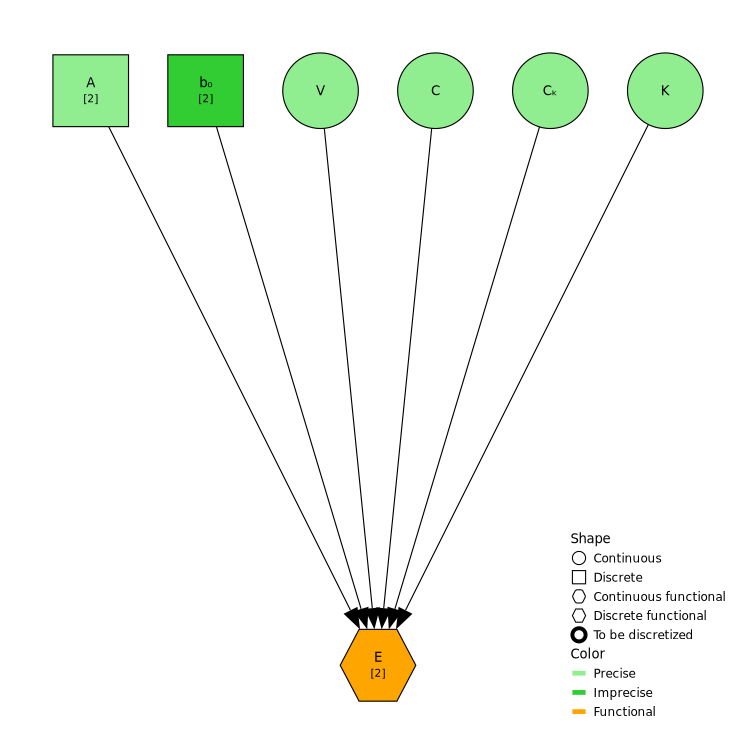

elapsed = @elapsed cn = reduce(ebn)
println("network reduced in ", round(elapsed; digits = 3), " s")

network reduced in 0.644 s

gplot(cn, background_color = "white", node_scale = 1.1, title = "Reduced Credal Network", label_size = 12)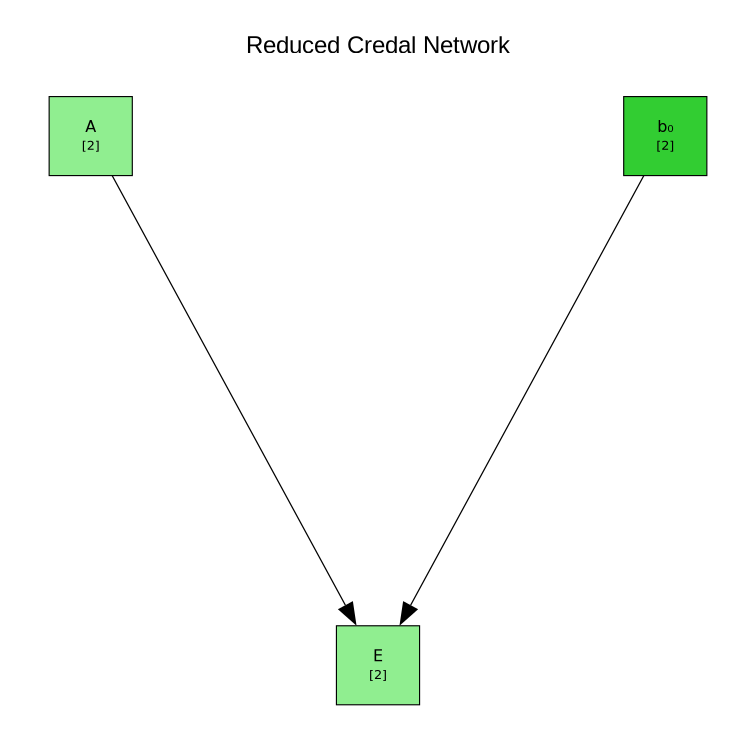

Because b₀ stayed imprecise, reduce returns a CredalNetwork, and the collapse probability inherits that imprecision: querying E gives lower and upper bounds.

infer(cn, :E, Evidence())

CredalPosterior P(E)

E	Interval
------------------------
E_failed	[0.027924, 0.041456]
E_safe	[0.958544, 0.972076]

Extreme posteriors: 2

---

This page was generated using Literate.jl.