
Vehicle Suspension Reliability
This example reproduces the vehicle-suspension reliability benchmark of Gerasimov & Vořechovský [19]. They do not build a Bayesian Network for it — they use it as a plain structural-reliability problem — so here it serves as a validation case: we cast the same problem as an enhanced Bayesian Network, reduce it, and check that the failure probability the network infers for a given scenario matches the one a direct Monte-Carlo reliability analysis returns for that same scenario.
The suspension's safety is governed by a composite limit state that combines four failure modes; the system fails as soon as any of them is violated. Two of the inputs are scenario variables handled as discrete nodes — the road coefficient and the load coefficient — while the vehicle speed and the suspension stiffness, tire stiffness and damping coefficient are continuous. All quantities follow the paper's unit system (a technical/CGS system, hence g = 981 cm/s²).
using EnhancedBayesianNetworksV precise and discretizable
In the standard benchmark the vehicle speed V is a precise root node with an ExactDiscretization: it is discretized exactly from its own distribution and, since everything else is precise, the network reduces to a plain Bayesian Network.
Fixed parameters
The sprung and unsprung masses and the gravitational acceleration are constants of the model.
M = 3.2633           # kg/cm/s²  (sprung mass)
m = 0.8158           # kg/cm/s²  (unsprung mass)
g = 981 # cm/s² (gravity)981Scenario nodes: road and load coefficients
The road coefficient (A, in rad·cm²/m) and the load coefficient (b₀, dimensionless) are discrete nodes. Each state carries a Parameter — the numerical value fed to the model when that state is active — so these nodes drive the scenario grid the reliability analysis is repeated over. The road / normal_load values (0.15915 / 0.27) are the deterministic values used in the paper.
A = DiscreteNode(:A, [:road => [Parameter(0.15915, :A)], :offroad => [Parameter(0.8, :A)]])  # A in rad·cm²/m
A[:A => :road] = 0.7
A[:A => :offroad] = 0.3

b₀ = DiscreteNode(:b₀, [:normal_load => [Parameter(0.27, :b₀)], :over_load => [Parameter(0.5, :b₀)]])
b₀[:b₀ => :normal_load] = 0.7
b₀[:b₀ => :over_load] = 0.30.3Vehicle speed
The speed V is a continuous root node, uniform between 7 and 12. Attaching an ExactDiscretization with explicit interval edges makes V survive the reduction as a discrete node (V_d), so we can later condition on a speed range. The edges span the full support [7, 12] so the bins match the distribution exactly, and the middle interval [9.5, 10.5] brackets the speed V = 10 used in the cross-check below.
discretization_v = ExactDiscretization([7.0, 8.5, 9.5, 10.5, 11.5, 12.0])  # edges in m/s
V = ContinuousNode(:V, Uniform(7, 12), discretization_v)                   # V in m/s
ContinuousNode: V
Parents: none
Discretization: ExactDiscretization
Intervals: 7.0, 8.5, 9.5, 10.5, 11.5, 12.0
Type: Precise
Support: [7.0, 12.0]
1×1 DataFrame
Row │ Π
│ Union…
─────┼─────────────────────────────────
1 │ Uniform{Float64}(a=7.0, b=12.0)Continuous suspension coefficients
The suspension stiffness C, the tire stiffness Cₖ and the damping coefficient K are continuous root nodes with normal distributions. They carry no discretization, so the reduction folds them into the failure model and integrates them out by simulation.
C = ContinuousNode(:C, Normal(431.7221, 10))     # kg/cm    (suspension stiffness)
Cₖ = ContinuousNode(:Cₖ, Normal(1475.5503, 10))   # kg/cm    (tire stiffness)
K = ContinuousNode(:K, Normal(55.0406, 10))       # kg/cm/s  (damping coefficient)
ContinuousNode: K
Parents: none
Type: Precise
Support: [-Inf, Inf]
1×1 DataFrame
Row │ Π
│ Union…
─────┼───────────────────────────────────
1 │ Normal{Float64}(μ=55.0406, σ=10.…The composite limit state
The four failure modes are, in order, exceedance of the road-holding ability (g1), exceedance of the rolling angle (g2), bumper hitting (g3) and exceedance of the minimum required tire life (g4). They are combined by taking their minimum: the suspension is failed when that minimum drops below zero (a series system — any single mode failing fails the whole). The performance function returns that minimum margin.
function composite_model(A, b₀, V, M, m, g, C, Cₖ, K)
    g1 = 1 .- (π .* m .* V .* A) ./ (b₀ .* K .* g .^ 2) .* [(Cₖ ./ (m .+ M) .- (C ./ M)) .^ 2 .+ C .^ 2 ./ (m .* M) .+ Cₖ .* K .^ 2 ./ (m .* M .^ 2)]
    g2 = 4000 .* C .* (M .* g) .^ (-1.5) .- 8.6394
    g3 = 2 .* .√(M .* g .* (K .^ 2 .* Cₖ ./ (C .* (m .+ M)) .+ C)) .- 1
    g4 = Cₖ .- [g .* (M .+ m)] .^ 0.877
    return minimum([g1[1], g2, g3, g4[1]])
end

model = Model(df -> composite_model.(df.A, df.b₀, df.V, M, m, g, df.C, df.Cₖ, df.K), :y)
performance = df -> df.y
#5 (generic function with 1 method)Building the enhanced Bayesian Network
The failure event E is a DiscreteFunctionalNode built from the limit-state model and its performance function; the six inputs (A, b₀, V, C, Cₖ, K) are its parents. A Monte-Carlo simulation propagates the continuous inputs' uncertainty through the model.
sim = MonteCarlo(10^6)
E = DiscreteFunctionalNode(:E, [model], performance, sim)

nodes = [A, b₀, V, C, Cₖ, K, E]
ebn = EnhancedBayesianNetwork(nodes)
add_child!(ebn, [A, b₀, V, C, Cₖ, K], E)
order!(ebn)

gplot(ebn, background_color = "white", legend = true, label_size = 10, legend_x = 15, legend_y = 14)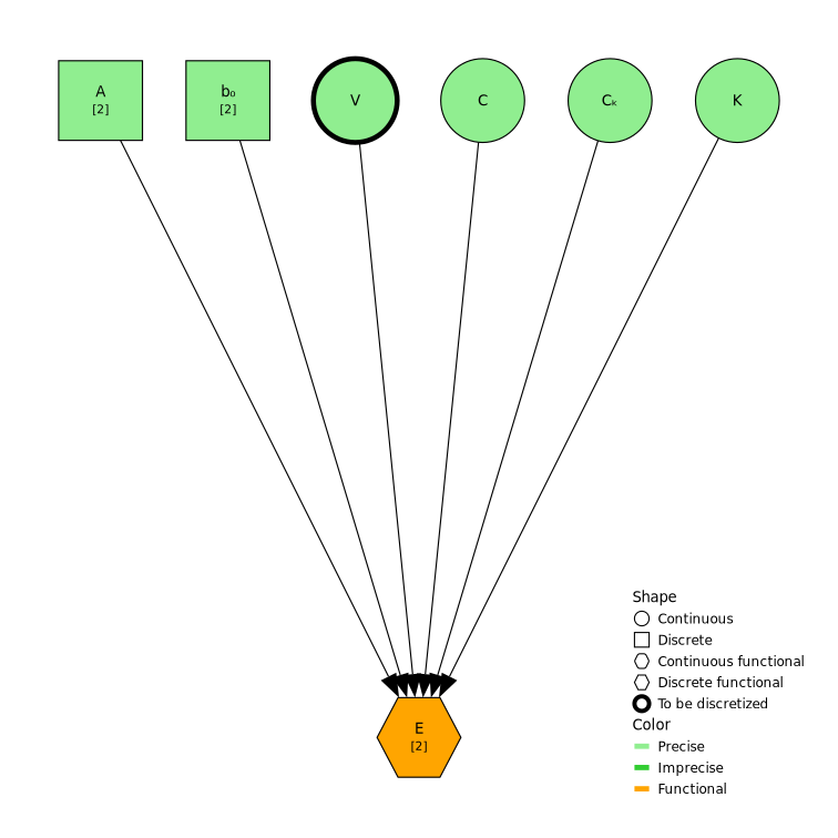
Reducing to a Bayesian Network
reduce evaluates the functional node: the continuous coefficients C, Cₖ, K are folded into the failure model and eliminated, while V — because it carries a discretization — is kept as a discrete node V_d. The result is a Bayesian Network over the road surface, the load, the discretized speed, and the collapse event. We time the reduction, as a rough indication measured on the machine building these docs:
elapsed = @elapsed bn = reduce(ebn)
println("network reduced in ", round(elapsed; digits = 3), " s")
network reduced in 10.049 sgplot(bn, background_color = "white", node_scale = 1.1, title = "Reduced Bayesian Network", label_size = 12)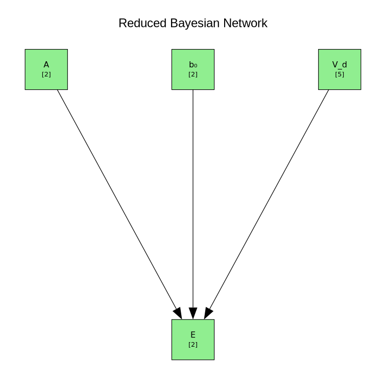
Inferring the failure probability for a scenario
With the network reduced, we can read off the probability of failure for a concrete scenario: driving on a normal-load road at a speed in the [9.5, 10.5] band (i.e. around V = 10).
evidence = Evidence(:V_d => Symbol("[9.5, 10.5]"), :A => :road, :b₀ => :normal_load)
elapsed = @elapsed ϕ = infer(bn, :E, evidence)
println("inference completed in ", round(elapsed; digits = 3), " s")
ϕ
Posterior P(E | V_d=[9.5, 10.5], b₀=normal_load, A=road)
E Probability
------------------------
E_failed 0.000526
E_safe 0.999474Cross-check against a direct reliability analysis
To confirm the network is faithful, we solve the same scenario directly with UncertaintyQuantification — fixing the road, load and speed to the scenario's values and running a Monte-Carlo estimate of the failure probability. This is the calculation Gerasimov & Vořechovský [19] perform; the enhanced Bayesian Network should reproduce it.
M = Parameter(3.2633, :M)                        # kg/cm/s²  (sprung mass)
m = Parameter(0.8158, :m)                        # kg/cm/s²  (unsprung mass)
g = Parameter(981, :g)                           # cm/s²     (gravity)
A = Parameter(0.15915, :A)                       # rad·cm²/m (road coefficient)
b₀ = Parameter(0.27, :b₀)                         # –         (load coefficient)
V = Parameter(10, :V)                            # m/s       (vehicle velocity)
C = RandomVariable(Normal(431.7221, 10), :C)     # kg/cm     (suspension stiffness)
Cₖ = RandomVariable(Normal(1475.5503, 10), :Cₖ)   # kg/cm     (tire stiffness)
K = RandomVariable(Normal(55.0406, 10), :K)      # kg/cm/s   (damping coefficient)

model = Model(df -> composite_model.(df.A, df.b₀, df.V, df.M, df.m, df.g, df.C, df.Cₖ, df.K), :y)
inputs = [A, b₀, V, M, m, g, C, Cₖ, K]

pf, cov, _ = probability_of_failure(model, performance, inputs, MonteCarlo(10^6))
(0.000584, 2.415903441779079e-5, 1000000×10 DataFrame
Row │ A b₀ V M m g C Cₖ ⋯
│ Float64 Float64 Float64 Float64 Float64 Float64 Float64 Floa ⋯
─────────┼──────────────────────────────────────────────────────────────────────
1 │ 0.15915 0.27 10.0 3.2633 0.8158 981.0 420.199 1454 ⋯
2 │ 0.15915 0.27 10.0 3.2633 0.8158 981.0 436.992 1462
3 │ 0.15915 0.27 10.0 3.2633 0.8158 981.0 429.415 1482
4 │ 0.15915 0.27 10.0 3.2633 0.8158 981.0 440.863 1471
5 │ 0.15915 0.27 10.0 3.2633 0.8158 981.0 420.348 1454 ⋯
6 │ 0.15915 0.27 10.0 3.2633 0.8158 981.0 427.734 1452
7 │ 0.15915 0.27 10.0 3.2633 0.8158 981.0 427.006 1478
8 │ 0.15915 0.27 10.0 3.2633 0.8158 981.0 444.82 1497
⋮ │ ⋮ ⋮ ⋮ ⋮ ⋮ ⋮ ⋮ ⋮ ⋱
999994 │ 0.15915 0.27 10.0 3.2633 0.8158 981.0 432.612 1460 ⋯
999995 │ 0.15915 0.27 10.0 3.2633 0.8158 981.0 433.035 1469
999996 │ 0.15915 0.27 10.0 3.2633 0.8158 981.0 410.523 1469
999997 │ 0.15915 0.27 10.0 3.2633 0.8158 981.0 430.88 1473
999998 │ 0.15915 0.27 10.0 3.2633 0.8158 981.0 449.582 1474 ⋯
999999 │ 0.15915 0.27 10.0 3.2633 0.8158 981.0 438.762 1477
1000000 │ 0.15915 0.27 10.0 3.2633 0.8158 981.0 447.004 1474
3 columns and 999985 rows omitted)The failure probability inferred by the Bayesian Network (the :E_failed entry of ϕ above) and the one from the direct Monte-Carlo analysis (pf) agree to within Monte-Carlo scatter — the network integrates the speed over the whole [9.5, 10.5] band while the direct check pins it to V = 10, so a small difference is expected. Both also match the reference value pF ≈ 5.2 × 10⁻⁴ that Gerasimov & Vořechovský [19] report for this configuration (from 10⁶ importance-sampling evaluations), confirming the enhanced Bayesian Network reproduces their result.
V imprecise and discretized
We now make V an imprecise root node — a p-box / interval — while keeping its discretization. Because V is a root, the discretization leaves the residual imprecise (unlike a child, whose residual is approximated to a precise distribution), so the imprecise speed still reaches the failure node E. The reliability analysis at E therefore stays a double-loop simulation, and the reduced network is a Credal Network.
The model, loads and coefficients are exactly those of the precise case; only V changes from a Uniform(7, 12) to an Interval(7, 12), and the failure node's simulation from a single-loop MonteCarlo to a DoubleLoop. (Everything is redefined here because the cross-check above rebound some of the node names to plain UncertaintyQuantification inputs.)
M = 3.2633           # kg/cm/s²  (sprung mass)
m = 0.8158           # kg/cm/s²  (unsprung mass)
g = 981              # cm/s²     (gravity)

A = DiscreteNode(:A, [:road => [Parameter(0.15915, :A)], :offroad => [Parameter(0.8, :A)]])  # A in rad·cm²/m
A[:A => :road] = 0.7
A[:A => :offroad] = 0.3

b₀ = DiscreteNode(:b₀, [:normal_load => [Parameter(0.27, :b₀)], :over_load => [Parameter(0.5, :b₀)]])
b₀[:b₀ => :normal_load] = 0.7
b₀[:b₀ => :over_load] = 0.3

discretization_v = ExactDiscretization([7.0, 9.5, 10.5, 12.0])  # edges in m/s (coarser bins)
V = ContinuousNode(:V, Interval(7, 12), discretization_v)       # V in m/s, imprecise

C = ContinuousNode(:C, Normal(431.7221, 10))     # kg/cm    (suspension stiffness)
Cₖ = ContinuousNode(:Cₖ, Normal(1475.5503, 10))   # kg/cm    (tire stiffness)
K = ContinuousNode(:K, Normal(55.0406, 10))       # kg/cm/s  (damping coefficient)

function composite_model(A, b₀, V, M, m, g, C, Cₖ, K)
    g1 = 1 .- (π .* m .* V .* A) ./ (b₀ .* K .* g .^ 2) .* [(Cₖ ./ (m .+ M) .- (C ./ M)) .^ 2 .+ C .^ 2 ./ (m .* M) .+ Cₖ .* K .^ 2 ./ (m .* M .^ 2)]
    g2 = 4000 .* C .* (M .* g) .^ (-1.5) .- 8.6394
    g3 = 2 .* .√(M .* g .* (K .^ 2 .* Cₖ ./ (C .* (m .+ M)) .+ C)) .- 1
    g4 = Cₖ .- [g .* (M .+ m)] .^ 0.877
    return minimum([g1[1], g2, g3, g4[1]])
end

model = Model(df -> composite_model.(df.A, df.b₀, df.V, M, m, g, df.C, df.Cₖ, df.K), :y)
performance = df -> df.y
#14 (generic function with 1 method)Building the enhanced Bayesian Network
Same wiring as before; only the failure node's simulation changes to a DoubleLoop, which propagates the imprecise speed with an outer loop over its interval and an inner reliability analysis. Because collapse is a rare event, the inner loop uses a SubSetSimulation rather than plain Monte Carlo, and the discretization above is kept coarse — a double loop is far more expensive than the single loop of the precise case.
sim = DoubleLoop(SubSetSimulation(100, 0.1, 10, Uniform(-0.2, 0.2)))
E = DiscreteFunctionalNode(:E, [model], performance, sim)

nodes = [A, b₀, V, C, Cₖ, K, E]
ebn = EnhancedBayesianNetwork(nodes)
add_child!(ebn, [A, b₀, V, C, Cₖ, K], E)
order!(ebn)

gplot(ebn, background_color = "white", legend = true, label_size = 10, legend_x = 15, legend_y = 14)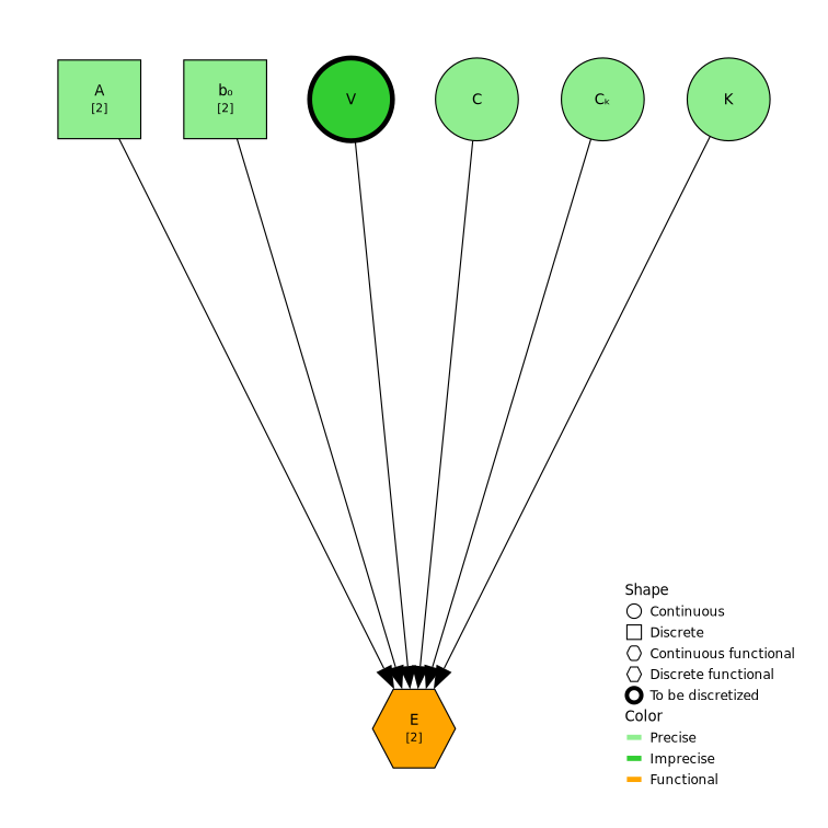
Reducing to a Credal Network
The discretized imprecise V is kept as V_d; its imprecise residual feeds E, whose double-loop analysis yields interval failure probabilities, so reduce returns a Credal Network. We time the reduction, as before:
elapsed = @elapsed cn = reduce(ebn)
println("network reduced in ", round(elapsed; digits = 3), " s")
network reduced in 16.691 sgplot(cn, background_color = "white", node_scale = 1.1, title = "Reduced Credal Network", label_size = 12)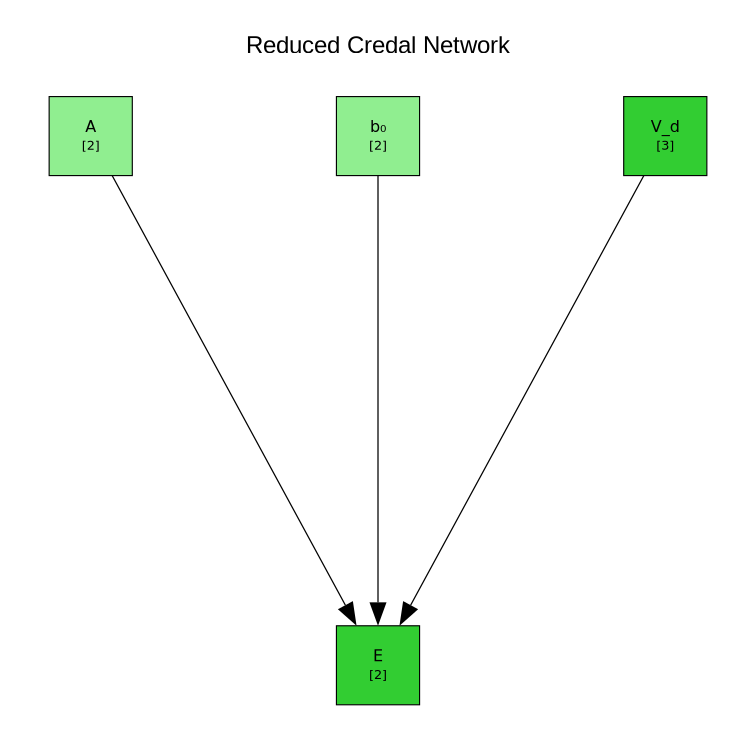
Inferring the failure probability for a scenario
The same scenario — a normal-load road at a speed in the [9.5, 10.5] band — now returns lower and upper bounds on the collapse probability:
evidence = Evidence(:V_d => Symbol("[9.5, 10.5]"), :A => :road, :b₀ => :normal_load)
elapsed = @elapsed ϕ = infer(cn, :E, evidence)
println("inference completed in ", round(elapsed; digits = 3), " s")
ϕ
CredalPosterior P(E | V_d=[9.5, 10.5], b₀=normal_load, A=road)
E Interval
------------------------
E_failed [4.18e-9, 0.01]
E_safe [0.99, 1.0]
Extreme posteriors: 4096 (8192 discarded: P(evidence) = 0)This page was generated using Literate.jl.