
Imprecision on a Continuous Node
The vehicle suspension example treats every input as precise. Here we revisit the same benchmark of Gerasimov & Vořechovský [19] — same model, loads and coefficients — but make the vehicle speed V imprecise: instead of a distribution, each road condition fixes V only to an interval (a p-box with unknown shape). This example shows how EnhancedBayesianNetworks propagates that imprecision, and — importantly — which simulation each modelling choice requires.
Two choices decide how the imprecision reaches the failure node and how it must be simulated:
whether
Vcarries a discretization, andwhether the functional node is discrete (a reliability analysis) or continuous (a distribution/p-box that is reconstructed).
The four cases below walk through the combinations.
using EnhancedBayesianNetworksThe shared model
The masses, gravity, road/load scenario nodes, the three precise suspension coefficients and the composite limit state are exactly those of the precise example; only V will change from case to case, so we define everything else once.
M = 3.2633           # kg/cm/s²  (sprung mass)
m = 0.8158           # kg/cm/s²  (unsprung mass)
g = 981              # cm/s²     (gravity)

A = DiscreteNode(:A, [:road => [Parameter(0.15915, :A)], :offroad => [Parameter(0.8, :A)]])  # A in rad·cm²/m
A[:A => :road] = 0.7
A[:A => :offroad] = 0.3

b₀ = DiscreteNode(:b₀, [:normal_load => [Parameter(0.27, :b₀)], :over_load => [Parameter(0.5, :b₀)]])
b₀[:b₀ => :normal_load] = 0.7
b₀[:b₀ => :over_load] = 0.3

C = ContinuousNode(:C, Normal(431.7221, 10))     # kg/cm    (suspension stiffness)
Cₖ = ContinuousNode(:Cₖ, Normal(1475.5503, 10))   # kg/cm    (tire stiffness)
K = ContinuousNode(:K, Normal(55.0406, 10))       # kg/cm/s  (damping coefficient)

function composite_model(A, b₀, V, M, m, g, C, Cₖ, K)
    g1 = 1 .- (π .* m .* V .* A) ./ (b₀ .* K .* g .^ 2) .* [(Cₖ ./ (m .+ M) .- (C ./ M)) .^ 2 .+ C .^ 2 ./ (m .* M) .+ Cₖ .* K .^ 2 ./ (m .* M .^ 2)]
    g2 = 4000 .* C .* (M .* g) .^ (-1.5) .- 8.6394
    g3 = 2 .* .√(M .* g .* (K .^ 2 .* Cₖ ./ (C .* (m .+ M)) .+ C)) .- 1
    g4 = Cₖ .- [g .* (M .+ m)] .^ 0.877
    return minimum([g1[1], g2, g3, g4[1]])
end

model = Model(df -> composite_model.(df.A, df.b₀, df.V, M, m, g, df.C, df.Cₖ, df.K), :y)
performance = df -> df.y
#5 (generic function with 1 method)V is imprecise: on a road its speed lies in [11, 13] m/s, off-road in [6, 8] m/s, with no assumed distribution inside those bands.
v_road = Interval(11, 13)      # m/s
v_offroad = Interval(6, 8)     # m/s
[6, 8]Case 1 — imprecise V, no discretization, feeding a discrete functional node: double-loop
When V is not discretized it reaches the failure node E as an imprecise continuous input. The reliability analysis at E therefore has to explore that imprecision, which is exactly what a DoubleLoop simulation does: an outer loop over the interval and an inner Monte-Carlo loop. The reduced network is credal, and E's own conditional probability table is interval-valued — a lower and upper failure probability per scenario.
V = ContinuousNode(:V, [:A])
V[:A => :road] = v_road
V[:A => :offroad] = v_offroad

E = DiscreteFunctionalNode(:E, [model], performance, DoubleLoop(MonteCarlo(10^3)))

ebn = EnhancedBayesianNetwork([A, b₀, V, C, Cₖ, K, E])
add_child!(ebn, A, V)
add_child!(ebn, [A, b₀, V, C, Cₖ, K], E)
order!(ebn)

gplot(ebn, background_color = "white", legend = true, label_size = 10, legend_x = 15, legend_y = 14)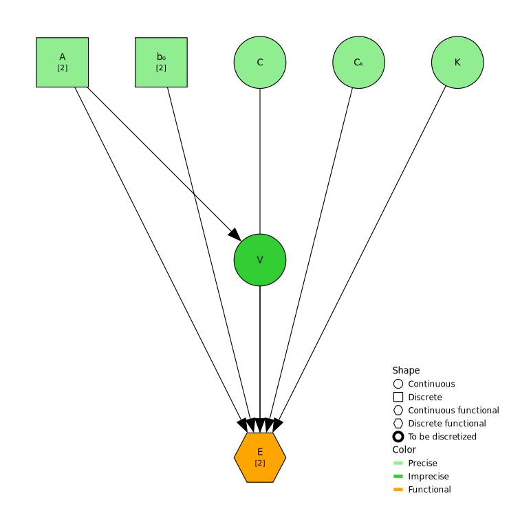
elapsed = @elapsed cn = reduce(ebn)
println("network reduced in ", round(elapsed; digits = 3), " s")
network reduced in 1.98 sThe failure node's table now carries intervals — the bounds on the collapse probability for each road/load scenario:
cn.nodes[findfirst(n -> n.name == :E, cn.nodes)].cpt.data| Row | b₀ | A | E | Π |
|---|---|---|---|---|
| Symbol | Symbol | Symbol | Union… | |
| 1 | normal_load | road | E_failed | [0.0, 0.003] |
| 2 | normal_load | road | E_safe | [0.997, 1.0] |
| 3 | normal_load | offroad | E_failed | [0.0, 0.004] |
| 4 | normal_load | offroad | E_safe | [0.996, 1.0] |
| 5 | over_load | road | E_failed | [0.0, 0.003] |
| 6 | over_load | road | E_safe | [0.997, 1.0] |
| 7 | over_load | offroad | E_failed | [0.0, 0.0015102805479251513] |
| 8 | over_load | offroad | E_safe | [0.9984897194520749, 1.0] |
gplot(cn, background_color = "white", node_scale = 1.1, title = "Reduced Credal Network", label_size = 12)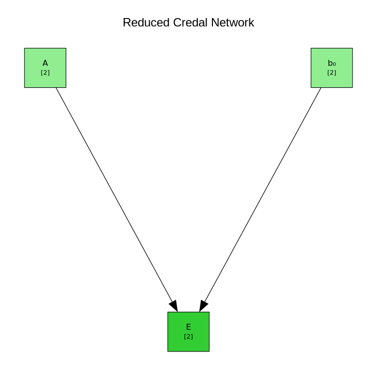
Case 2 — imprecise V, discretized, feeding a discrete functional node: single-loop
Attaching an ApproximatedDiscretization to V changes the picture. During reduction an imprecise continuous node is split: its imprecision moves into the discrete surrogate V_d (whose bin probabilities become intervals — a credal node), while the continuous residual handed to E is approximated by a precise distribution. So E no longer sees any imprecise continuous input.
discretization_v = ApproximatedDiscretization([6.0, 8.0, 10.0, 13.0], 2)  # edges in m/s

V = ContinuousNode(:V, [:A], discretization_v)
V[:A => :road] = v_road
V[:A => :offroad] = v_offroad

E = DiscreteFunctionalNode(:E, [model], performance, DoubleLoop(MonteCarlo(10^6)))

ebn = EnhancedBayesianNetwork([A, b₀, V, C, Cₖ, K, E])
add_child!(ebn, A, V)
add_child!(ebn, [A, b₀, V, C, Cₖ, K], E)
order!(ebn)

gplot(ebn, background_color = "white", legend = true, label_size = 10, legend_x = 15, legend_y = 14)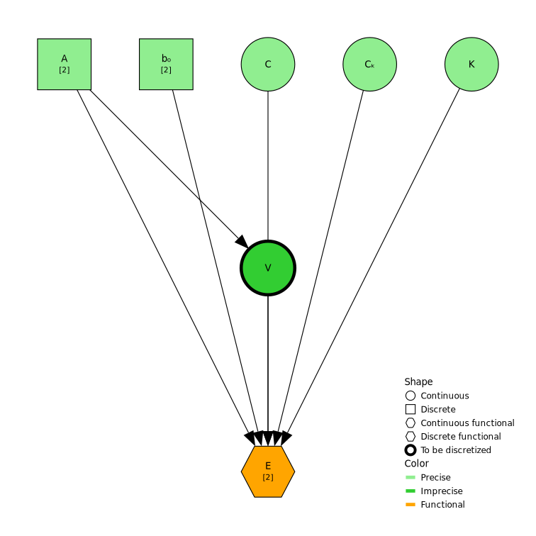
Because E's inputs are now precise, a DoubleLoop has nothing imprecise to loop over and the reduction raises an error. We catch it here to show the message:
try
    reduce(ebn)
catch e
    showerror(stdout, e)
end
Invalid simulation for functional node :E: the assigned DoubleLoop is an imprecise (double-loop) simulation, but every input reaching :E is precise. This happens when an imprecise continuous ancestor of :E is discretized: discretization moves the imprecision into the discrete (credal) surrogate node and leaves a precise continuous residual feeding :E. Use a single-loop simulation (e.g. MonteCarlo) for :E; the network stays credal through the discretized node. Alternatively, remove the discretization from the imprecise continuous ancestor so its imprecision reaches :E directly.Single-loop after discretizing an imprecise child node
When the only imprecision feeding a functional node comes from a non-root imprecise continuous ancestors that are discretized, use a single-loop simulation (e.g. MonteCarlo). Discretization has already carried the imprecision into the credal discrete surrogate; the residual reaching the functional node is precise, so a double loop is neither needed nor valid.
Swapping the simulation to a single-loop MonteCarlo fixes it. The imprecision is not lost — it now lives in the credal V_d, so the reduced network is still a CredalNetwork:
V = ContinuousNode(:V, [:A], discretization_v)
V[:A => :road] = v_road
V[:A => :offroad] = v_offroad

E = DiscreteFunctionalNode(:E, [model], performance, MonteCarlo(10^6))

ebn = EnhancedBayesianNetwork([A, b₀, V, C, Cₖ, K, E])
add_child!(ebn, A, V)
add_child!(ebn, [A, b₀, V, C, Cₖ, K], E)
order!(ebn)

elapsed = @elapsed cn = reduce(ebn)
println("network reduced in ", round(elapsed; digits = 3), " s")
network reduced in 3.999 sgplot(cn, background_color = "white", node_scale = 1.1, title = "Reduced Credal Network", label_size = 12)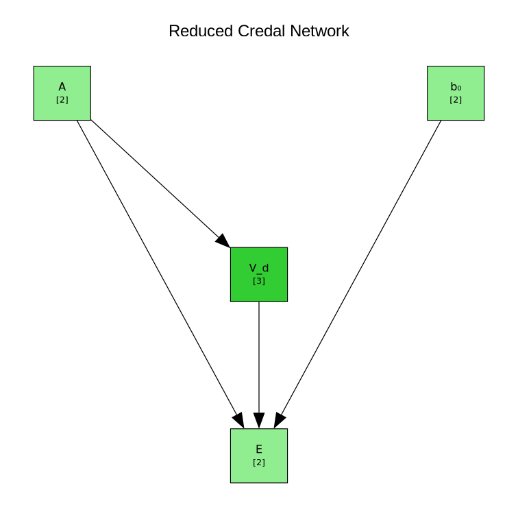
Case 3 — imprecise V, no discretization, feeding a continuous functional node: MonteCarlo
When the functional node is continuous rather than discrete, imprecision is handled differently again. Leaving V imprecise (no discretization), a ContinuousFunctionalNode propagates it with an ordinary MonteCarlo and reconstructs the output as a probability box — a lower/upper distribution pair. Continuous functional nodes have no double-loop variant, so a single-loop MonteCarlo is the right (and only) choice: this is the continuous counterpart of Case 1.
V = ContinuousNode(:V, [:A])
V[:A => :road] = v_road
V[:A => :offroad] = v_offroad

E = ContinuousFunctionalNode(:E, [model], MonteCarlo(10^6))

ebn = EnhancedBayesianNetwork([A, b₀, V, C, Cₖ, K, E])
add_child!(ebn, A, V)
add_child!(ebn, [A, b₀, V, C, Cₖ, K], E)
order!(ebn)

gplot(ebn, background_color = "white", legend = true, label_size = 10, legend_x = 15, legend_y = 14)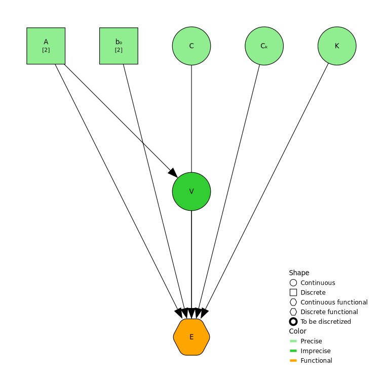
elapsed = @elapsed cn = reduce(ebn)
println("network reduced in ", round(elapsed; digits = 3), " s")
network reduced in 5.204 sgplot(cn, background_color = "white", node_scale = 1.1, title = "Reduced Credal Network", label_size = 12)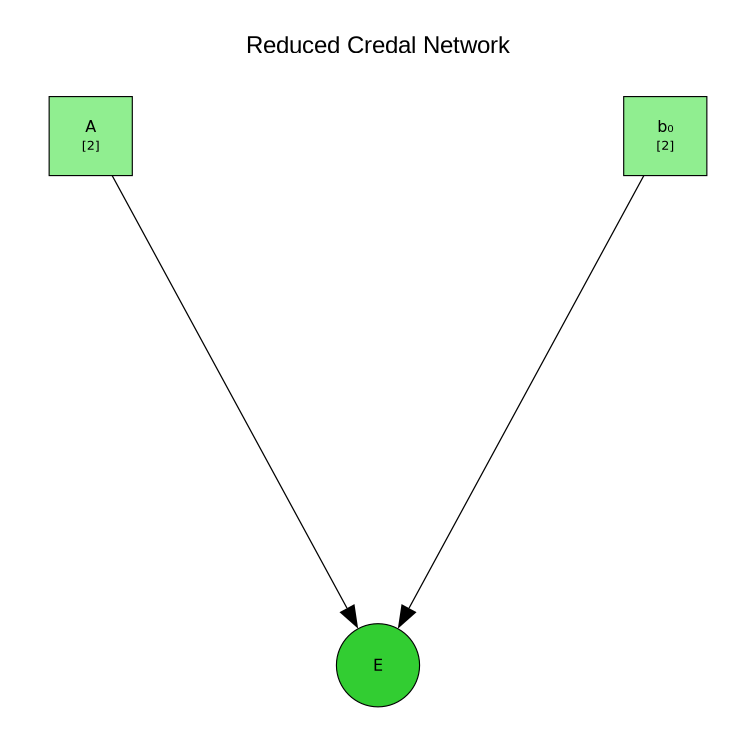
The failure node is now a continuous node whose entries are :lb/:ub EmpiricalDistribution pairs — the reconstructed p-box:
cn.nodes[findfirst(n -> n.name == :E, cn.nodes)].cpt.data| Row | b₀ | A | Π |
|---|---|---|---|
| Symbol | Symbol | Union… | |
| 1 | normal_load | road | Pair{Symbol, EmpiricalDistribution}[:lb=>EmpiricalDistribution( data: [0.757554, 0.773179, 0.40682, 0.588589, 0.79748, 0.764122, 0.775643, 0.51769, 0.718865, 0.727296 … 0.646638, 0.713397, 0.68502, 0.790834, 0.722157, 0.729145, 0.79533, 0.769156, 0.666996, 0.724099] lb: 0.326846 ub: 0.878813 h: 0.0078425 c: Spline1D(knots=[0.326846,0.326901 … 0.878758,0.878813] (10000 elements), k=1, extrapolation="nearest", residual=0.0) q: Spline1D(knots=[0.0,1.26274e-20 … 1.0,1.0] (9828 elements), k=1, extrapolation="nearest", residual=0.0) ) , :ub=>EmpiricalDistribution( data: [0.794853, 0.773179, 0.40682, 0.588589, 0.828637, 0.800411, 0.81016, 0.51769, 0.762117, 0.727296 … 0.646638, 0.75749, 0.68502, 0.823013, 0.764902, 0.770815, 0.826818, 0.80467, 0.666996, 0.724099] lb: 0.306607 ub: 0.928049 h: 0.0102884 c: Spline1D(knots=[0.306607,0.30667 … 0.927987,0.928049] (10000 elements), k=1, extrapolation="nearest", residual=0.0) q: Spline1D(knots=[0.0,1.41553e-20 … 1.0,1.0] (9827 elements), k=1, extrapolation="nearest", residual=0.0) ) ] |
| 2 | normal_load | offroad | Pair{Symbol, EmpiricalDistribution}[:lb=>EmpiricalDistribution( data: [0.416908, 0.320602, 0.356193, 0.394918, 0.195576, 0.128073, 0.302443, 0.275541, 0.305327, 0.192246 … 0.383275, 0.107095, 0.345491, 0.265808, 0.323115, 0.284857, 0.184531, 0.234137, 0.396274, 0.265856] lb: -0.0847414 ub: 0.55397 h: 0.0164666 c: Spline1D(knots=[-0.0847414,-0.0846776 … 0.553906,0.55397] (10000 elements), k=1, extrapolation="nearest", residual=0.0) q: Spline1D(knots=[0.0,1.4415e-20 … 1.0,1.0] (9728 elements), k=1, extrapolation="nearest", residual=0.0) ) , :ub=>EmpiricalDistribution( data: [0.548248, 0.490452, 0.517144, 0.546188, 0.396682, 0.346055, 0.476832, 0.456656, 0.478995, 0.394184 … 0.537456, 0.330321, 0.509118, 0.449356, 0.492336, 0.463643, 0.388398, 0.425603, 0.547205, 0.449392] lb: 0.188713 ub: 0.657192 h: 0.0120228 c: Spline1D(knots=[0.188713,0.18876 … 0.657146,0.657192] (10000 elements), k=1, extrapolation="nearest", residual=0.0) q: Spline1D(knots=[0.0,1.05746e-20 … 1.0,1.0] (9719 elements), k=1, extrapolation="nearest", residual=0.0) ) ] |
| 3 | over_load | road | Pair{Symbol, EmpiricalDistribution}[:lb=>EmpiricalDistribution( data: [0.854959, 0.843505, 0.851897, 0.702569, 0.871234, 0.856338, 0.663427, 0.879141, 0.870929, 0.833125 … 0.897684, 0.731975, 0.869021, 0.898108, 0.861531, 0.870102, 0.638143, 0.878264, 0.728482, 0.8809] lb: 0.0199821 ub: 0.963656 h: 0.0077354 c: Spline1D(knots=[0.0199821,0.0200765 … 0.963562,0.963656] (10000 elements), k=1, extrapolation="nearest", residual=0.0) q: Spline1D(knots=[0.0,2.20684e-20 … 1.0,1.0] (7340 elements), k=1, extrapolation="nearest", residual=0.0) ) , :ub=>EmpiricalDistribution( data: [0.854959, 0.843505, 0.874682, 0.702569, 0.891044, 0.87844, 0.663427, 0.897735, 0.890786, 0.833125 … 0.913425, 0.731975, 0.889171, 0.913784, 0.882834, 0.890086, 0.638143, 0.896993, 0.728482, 0.899223] lb: 0.0263744 ub: 0.972907 h: 0.00696519 c: Spline1D(knots=[0.0263744,0.0264691 … 0.972813,0.972907] (10000 elements), k=1, extrapolation="nearest", residual=0.0) q: Spline1D(knots=[0.0,2.22692e-20 … 1.0,1.0] (7234 elements), k=1, extrapolation="nearest", residual=0.0) ) ] |
| 4 | over_load | offroad | Pair{Symbol, EmpiricalDistribution}[:lb=>EmpiricalDistribution( data: [0.63808, 0.655901, 0.117159, 0.589395, 0.595246, 0.625501, 0.568261, 0.601152, 0.614489, 0.521597 … 0.590393, 0.612981, 0.426267, 0.649709, 0.591894, 0.616983, 0.571704, 0.624706, 0.649442, 0.573827] lb: -3.18592 ub: 0.813543 h: 0.0157608 c: Spline1D(knots=[-3.18592,-3.18552 … 0.813143,0.813543] (10000 elements), k=1, extrapolation="nearest", residual=0.0) q: Spline1D(knots=[0.0,9.88855e-20 … 1.0,1.0] (2673 elements), k=1, extrapolation="nearest", residual=0.0) ) , :ub=>EmpiricalDistribution( data: [0.72856, 0.716232, 0.117159, 0.692046, 0.696435, 0.719126, 0.676196, 0.700864, 0.710867, 0.641198 … 0.692795, 0.709736, 0.426267, 0.737282, 0.69392, 0.712737, 0.678778, 0.718529, 0.737081, 0.68037] lb: -3.15351 ub: 0.860559 h: 0.01182 c: Spline1D(knots=[-3.15351,-3.15311 … 0.860158,0.860559] (10000 elements), k=1, extrapolation="nearest", residual=0.0) q: Spline1D(knots=[0.0,1.03063e-19 … 1.0,1.0] (2407 elements), k=1, extrapolation="nearest", residual=0.0) ) ] |
Case 4 — imprecise V, discretized, feeding a continuous functional node: MonteCarlo
The final combination discretizes V and feeds a continuous functional node — the continuous counterpart of Case 2. Discretization again splits V: the imprecision moves into the credal V_d, and the residual reaching E is precise. So the continuous functional node has only precise inputs and reconstructs a single precise distribution (not a p-box); a single-loop MonteCarlo is all that is needed, and the imprecision survives in V_d.
V = ContinuousNode(:V, [:A], discretization_v)
V[:A => :road] = v_road
V[:A => :offroad] = v_offroad

E = ContinuousFunctionalNode(:E, [model], MonteCarlo(500))

ebn = EnhancedBayesianNetwork([A, b₀, V, C, Cₖ, K, E])
add_child!(ebn, A, V)
add_child!(ebn, [A, b₀, V, C, Cₖ, K], E)
order!(ebn)

gplot(ebn, background_color = "white", legend = true, label_size = 10, legend_x = 15, legend_y = 14)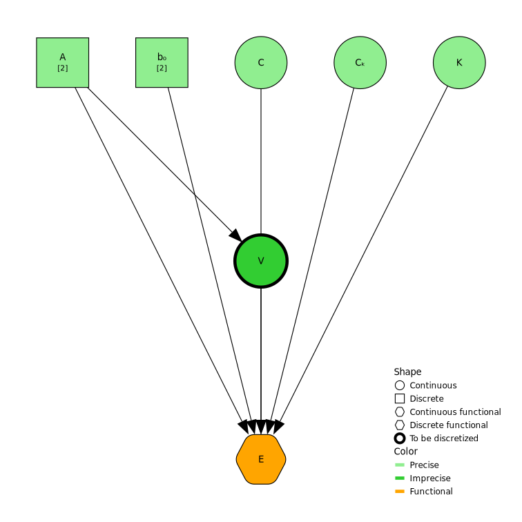
elapsed = @elapsed cn = reduce(ebn)
println("network reduced in ", round(elapsed; digits = 3), " s")
network reduced in 7.596 sgplot(cn, background_color = "white", node_scale = 1.1, title = "Reduced Credal Network", label_size = 12)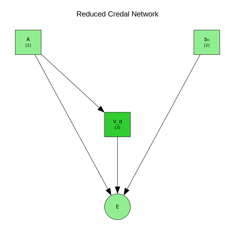
Unlike Case 3, E is now a single precise distribution; the imprecision instead lives in the discretized node V_d, whose bin probabilities are intervals:
cn.nodes[findfirst(n -> n.name == :V_d, cn.nodes)].cpt.data| Row | A | V_d | Π |
|---|---|---|---|
| Symbol | Symbol | Union… | |
| 1 | road | [6.0, 8.0] | [0, 1] |
| 2 | offroad | [6.0, 8.0] | [0, 1] |
| 3 | road | [8.0, 10.0] | [0, 1] |
| 4 | offroad | [8.0, 10.0] | [0, 1] |
| 5 | road | [10.0, 13.0] | [0, 1] |
| 6 | offroad | [10.0, 13.0] | [0, 1] |
This page was generated using Literate.jl.